Open in molab View on GitHub Download .py

Propagating uncertainty using Monte-Carlo simulations¶

The analytical law of propagation (RSS with sensitivity coefficients) has three limits:

It is exact only for linear measurement functions.
It assumes the output is normally distributed.
Complex models invite algebra mistakes when combining terms.

Monte-Carlo (MC) propagation skips the algebra: draw many random input sets from their distributions, push each through \(y = f(x)\), and read the output distribution directly — mean, standard deviation, and any coverage interval.

import numpy as np
import matplotlib.pyplot as plt

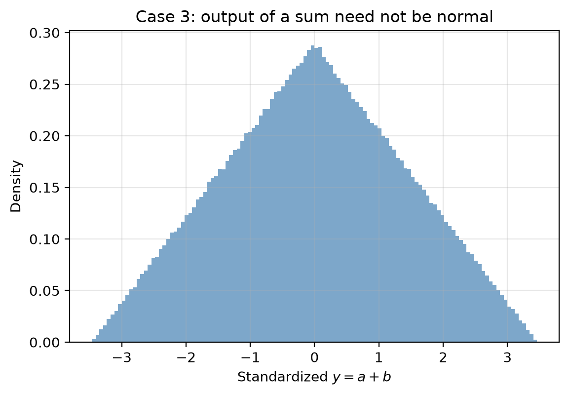
Interactive: what does \(y = a + b\) look like?¶

Even the simplest sum produces different output shapes depending on the inputs. Drag the slider through the 6 cases (\(10^6\) trials each, seed 42):

normal + normal, equal size → normal output
normal + wider normal → still normal, wider
uniform + uniform, equal size → triangular output
uniform + wider uniform → complex (trapezoidal) output
normal + uniform → complex output, hard to predict
normal + wider uniform → complex output

How simulation works¶

Define the measurement function \(y = f(x)\), with \(x\) a vector of influence quantities.
Draw \(m\) random input sets from each input's distribution (normal, rectangular, …).
Push every set through \(f\): \(Y = f(X)\).
Read the output: mean, standard deviation, and percentiles for the coverage interval (e.g. 2.5th/97.5th for 95%).

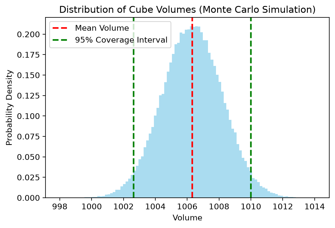
Example 1: non-linear propagation — cube volume \(V = h^3\)¶

def monte_carlo_cube_volume(measurements, resolution, num_simulations=100000):
    # Calculate mean and standard deviation of measurements
    mean_height = np.mean(measurements)
    std_height = np.std(measurements, ddof=1)

    # Type B uncertainty (assuming rectangular distribution for resolution)
    u_b = resolution / np.sqrt(3)

    # Combine Type A and Type B uncertainties
    u_c = np.sqrt((std_height / np.sqrt(len(measurements)))**2 + u_b**2)

    # Generate Monte Carlo simulations
    simulated_heights = np.random.normal(mean_height, u_c, num_simulations)

    # Calculate volumes
    simulated_volumes = simulated_heights**3

    # Calculate results
    mean_volume = np.mean(simulated_volumes)
    std_volume = np.std(simulated_volumes)

    # Calculate coverage interval (95%)
    coverage_interval = np.percentile(simulated_volumes, [2.5, 97.5])

    print(f"Mean height: {mean_height:.6f}")
    print(f"Combined standard uncertainty of height: {u_c:.6f}")
    print(f"Mean volume: {mean_volume:.6f}")
    print(f"Standard uncertainty of volume: {std_volume:.6f}")
    print(f"95% coverage interval for volume: [{coverage_interval[0]:.6f}, {coverage_interval[1]:.6f}]")

    # Plot histogram of simulated volumes
    plt.figure(figsize=(6.4, 4.1))
    plt.hist(simulated_volumes, bins=100, density=True, alpha=0.7, color='skyblue')
    plt.axvline(mean_volume, color='red', linestyle='dashed', linewidth=2, label='Mean Volume')
    plt.axvline(coverage_interval[0], color='green', linestyle='dashed', linewidth=2, label='95% Coverage Interval')
    plt.axvline(coverage_interval[1], color='green', linestyle='dashed', linewidth=2)
    plt.xlabel('Volume')
    plt.ylabel('Probability Density')
    plt.title('Distribution of Cube Volumes (Monte Carlo Simulation)')
    plt.legend()
    plt.show()

# Example usage
height_measurements = [10.02, 10.03, 10.01, 10.02, 10.03, 10.02, 10.01, 10.02, 10.03, 10.02]
resolution = 0.01  # mm
monte_carlo_cube_volume(height_measurements, resolution)

Mean height: 10.021000
Combined standard uncertainty of height: 0.006227
Mean volume: 1006.315075
Standard uncertainty of volume: 1.880801
95% coverage interval for volume: [1002.626877, 1009.989970]

Example 2: thermal expansion — where first-order theory falls short¶

Measurement model: \(\Delta L = L \cdot \Delta T \cdot \alpha\).

First-order propagation gives \(u^2(\Delta L) = (\Delta T\alpha)^2u^2(L) + (L\alpha)^2u^2(\Delta T) + (L\Delta T)^2u^2(\alpha)\), but the exact expansion adds higher-order products such as \(\Delta T\,u^2(L)u^2(\alpha)\) and \(u^2(\Delta T)u^2(L)u^2(\alpha)\). A \(10^6\)-trial simulation of \((L, \Delta T, \alpha)\) needs none of that algebra and stays correct where the first-order approximation drifts — especially at 99.9% coverage, where the simulated range runs almost twice the first-order prediction.

Example 3: cosine error — a non-normal output¶

A 200 mm length measured with 2 µm length uncertainty and 1° alignment uncertainty produces a visibly non-normal output distribution. Theory and simulation agree on the standard uncertainty but disagree on the confidence limits — and the gap grows with the confidence level. This is exactly the case simulation exists for.

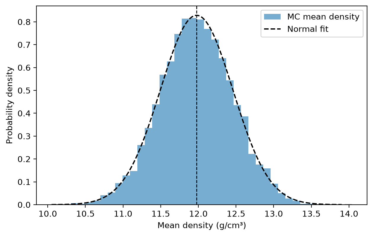
Example 4: real data — density from caliper, micrometer, and balance¶

Diameter (caliper, res 0.01 mm), height (micrometer, res 0.001 mm), and mass (balance, \(u = 0.1\) g) combine into density. Analytical relative propagation and a 5000-trial MC of the mean density agree — run both and compare.

Mean density = 11.9769 ± 0.4816 g/cm^3 (1σ, MC of the mean)

Best practices for simulation¶

Trials: use at least \(10^6\) trials; more for high confidence levels; check convergence by increasing the count.
Distributions: match actual measurement conditions and document every assumption.
Validation: compare against the analytical result where one exists, and check sensitivity to input parameters.
Documentation: record trial count, distributions, and confidence level with the result.