Statistical distribution
Let's have a look how different statistical distributions look like, to have a better idea what to use as prior on our inference bayesian exploration.
All the distributions available in scipy can be found on the docs here: http://docs.scipy.org/doc/scipy/reference/stats.html#module-scipy.stats
Let's start with Discrete distributions
Discrete Distributions
- bernoulli: A Bernoulli discrete random variable.
- binom: A binomial discrete random variable.
- poisson: A Poisson discrete random variable.
- ...
Exploring Different Probability Distributions
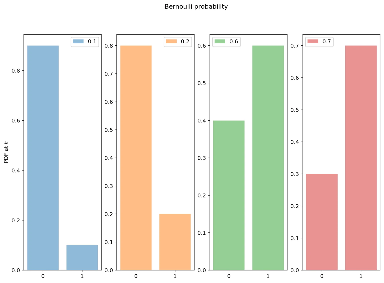
Bernoulli distribution
Given a certain probability \(p\), the Bernoulli distribution takes value \(k=1\), meanwhile it takes \(k=0\) in all the other cases \(1-p\).
In other words:
array([1, 1, 1, 1, 1, 1, 0, 1, 0, 1, 1, 0, 0, 1, 1, 1, 1, 0, 0, 1, 1, 0,
       1, 0, 1, 1, 1, 1, 1, 1, 1, 0, 1, 0, 1, 1, 0, 1, 0, 0, 1, 1, 0, 0,
       0, 0, 1, 1, 1, 1, 0, 1, 0, 1, 1, 1, 1, 0, 1, 1, 1, 1, 0, 1, 1, 1,
       1, 0, 0, 1, 0, 1, 0, 1, 1, 1, 1, 1, 0, 1, 1, 1, 0, 0, 0, 1, 1, 1,
       0, 1, 0, 0, 0, 0, 0, 0, 1, 1, 1, 0])
_a = np.arange(2)
colors = matplotlib.rcParams['axes.prop_cycle'].by_key()['color']
plt.figure(figsize=(12, 8))
for _i, _p in enumerate([0.1, 0.2, 0.6, 0.7]):
    ax = plt.subplot(1, 4, _i + 1)
    plt.bar(_a, bernoulli.pmf(_a, _p), label=_p, color=colors[_i], alpha=0.5)
    ax.xaxis.set_ticks(_a)
    plt.legend(loc=0)
    if _i == 0:
        plt.ylabel('PDF at $k$')
plt.suptitle('Bernoulli probability')
Poisson Distribution
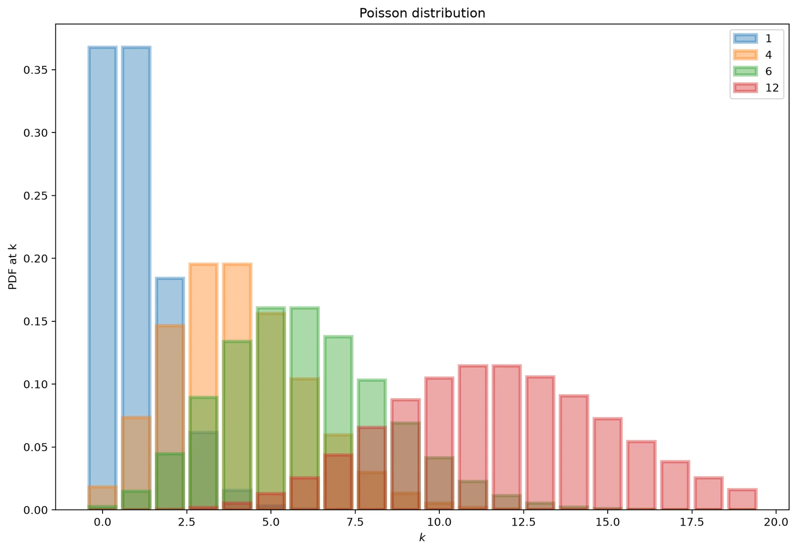
Another discrete distribution, the Poisson Distribution is defined for all the integer positive number as
_k = np.arange(20)
colors_1 = matplotlib.rcParams['axes.prop_cycle'].by_key()['color']
plt.figure(figsize=(12, 8))
for _i, _lambda_ in enumerate([1, 4, 6, 12]):
    plt.bar(_k, poisson.pmf(_k, _lambda_), label=_lambda_, color=colors_1[_i], alpha=0.4, edgecolor=colors_1[_i], lw=3)
    plt.legend()
plt.title('Poisson distribution')
plt.xlabel('$k$')
plt.ylabel('PDF at k')
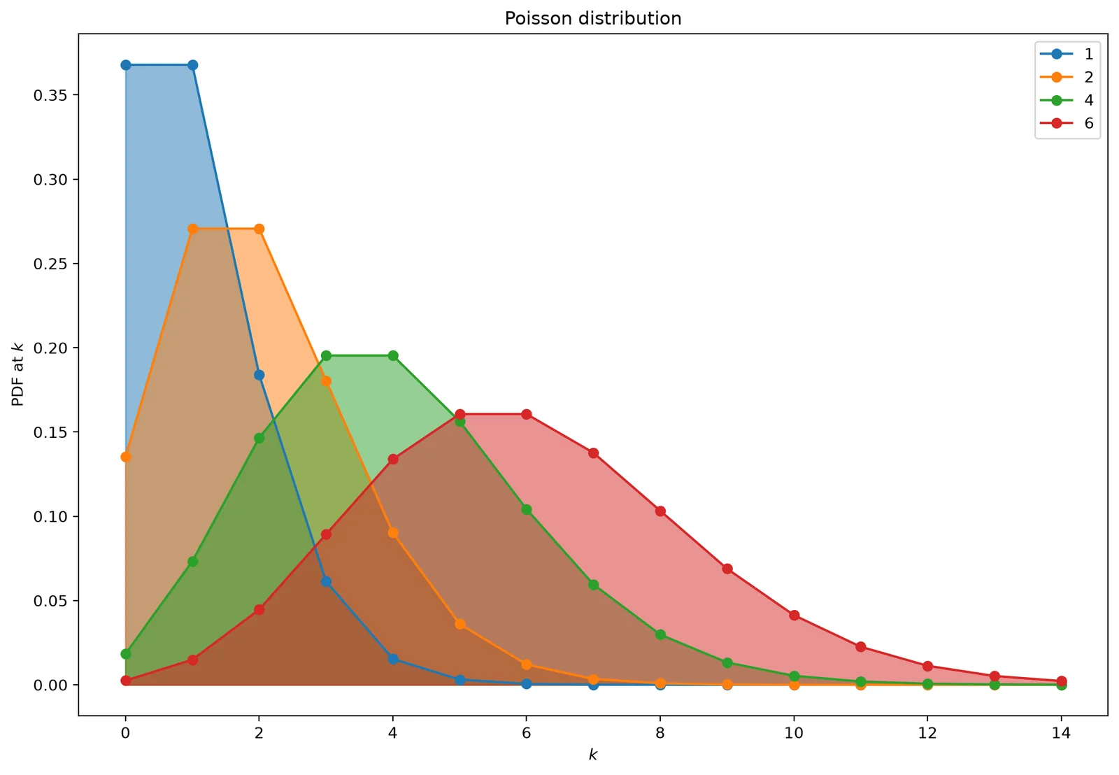
_k = np.arange(15)
plt.figure(figsize=(12, 8))
for _i, _lambda_ in enumerate([1, 2, 4, 6]):
    plt.plot(_k, poisson.pmf(_k, _lambda_), '-o', label=_lambda_, color=colors_1[_i])
    plt.fill_between(_k, poisson.pmf(_k, _lambda_), color=colors_1[_i], alpha=0.5)
    plt.legend()
plt.title('Poisson distribution')
plt.ylabel('PDF at $k$')
plt.xlabel('$k$')
Binomial distribution
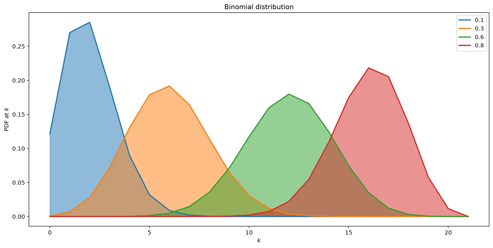
Last but not least, the binomial distribution which is defined as:
where
with \(k={1, 2, 3, \ldots}\)
plt.figure(figsize=(12, 6))
_k = np.arange(0, 22)
for _p, color in zip([0.1, 0.3, 0.6, 0.8], colors_1):
    rv = binom(20, _p)
    plt.plot(_k, rv.pmf(_k), lw=2, color=color, label=_p)
    plt.fill_between(_k, rv.pmf(_k), color=color, alpha=0.5)
plt.legend()
plt.title('Binomial distribution')
plt.tight_layout()
plt.ylabel('PDF at $k$')
plt.xlabel('$k$')
Continous Probability Distribution
They are defined for any value of a positive \(x\). A lot of distribution are defined on scipy.stats, so I will explore only som:
- alpha An alpha continuous random variable.
- beta A beta continuous random variable.
- gamma A gamma continuous random variable.
- expon An exponential continuous random variable.
- ...
Alpha
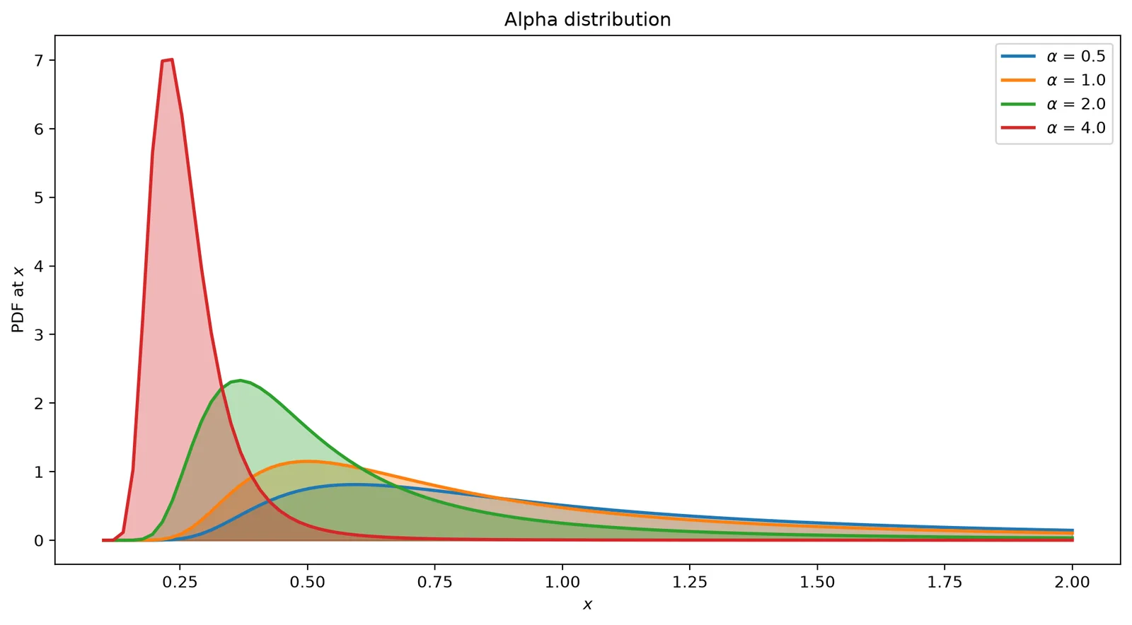
The Alpha distribution is defined as
_x = np.linspace(0.1, 2, 100)
alpha = scipy.stats.alpha
alphas = [0.5, 1, 2, 4]
plt.figure(figsize=(12, 6))
for _a, _c in zip(alphas, colors_1):
    label = '$\\alpha$ = {0:.1f}'.format(_a)
    plt.plot(_x, alpha.pdf(_x, _a), lw=2, color=_c, label=label)
    plt.fill_between(_x, alpha.pdf(_x, _a), color=_c, alpha=0.33)
plt.ylabel('PDF at $x$')
plt.xlabel('$x$')
plt.title('Alpha distribution')
plt.legend()
Beta distribution
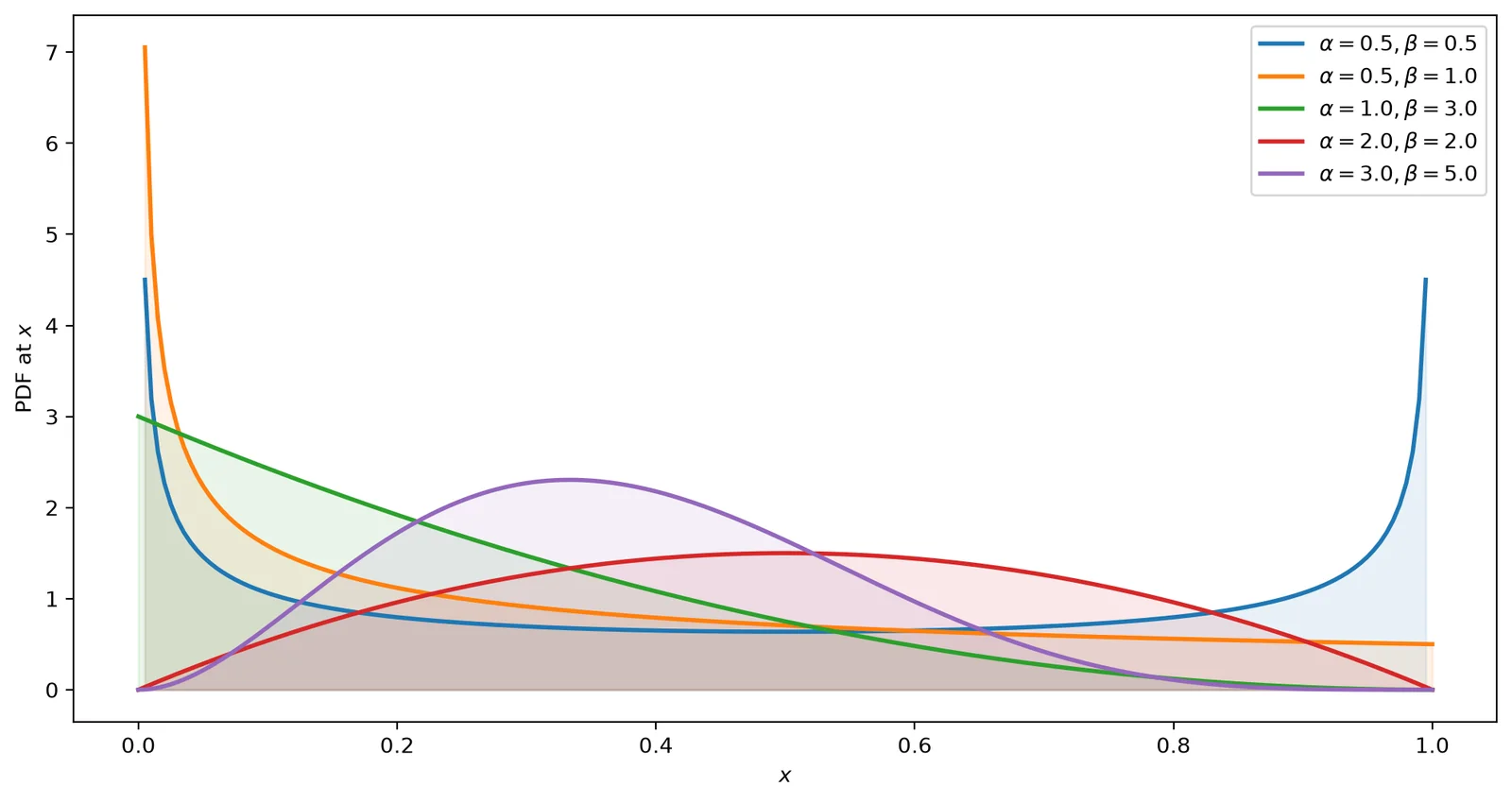
The Beta distribution is defined for a variabile rangin between 0 and 1.
The pdf is defined as:
beta = scipy.stats.beta
_x = np.linspace(0, 1, num=200)
fig = plt.figure(figsize=(12, 6))
for _a, b, _c in zip([0.5, 0.5, 1, 2, 3], [0.5, 1, 3, 2, 5], colors_1):
    plt.plot(_x, beta.pdf(_x, _a, b), lw=2, c=_c, label='$\\alpha = {0:.1f}, \\beta={1:.1f}$'.format(_a, b))
    plt.fill_between(_x, beta.pdf(_x, _a, b), color=_c, alpha=0.1)
plt.legend(loc=0)
plt.ylabel('PDF at $x$')
plt.xlabel('$x$')
Gamma distribution
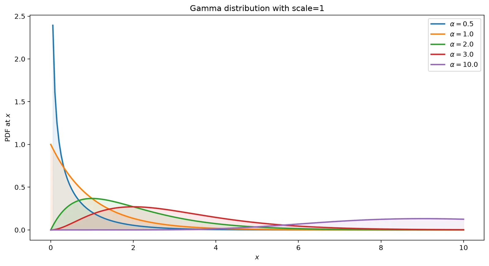
The gamma distribution uses the Gamma function (http://en.wikipedia.org/wiki/Gamma_function) and it has two shape parameters.
The scale parameter is equal = \(1.0/\lambda\)
gamma = scipy.stats.gamma
plt.figure(figsize=(12, 6))
_x = np.linspace(0, 10, num=200)
for _a, _c in zip([0.5, 1, 2, 3, 10], colors_1):
    plt.plot(_x, gamma.pdf(_x, _a), lw=2, c=_c, label='$\\alpha = {0:.1f}$'.format(_a))
    plt.fill_between(_x, gamma.pdf(_x, _a), color=_c, alpha=0.1)
plt.legend(loc=0)
plt.title('Gamma distribution with scale=1')
plt.ylabel('PDF at $x$')
plt.xlabel('$x$')
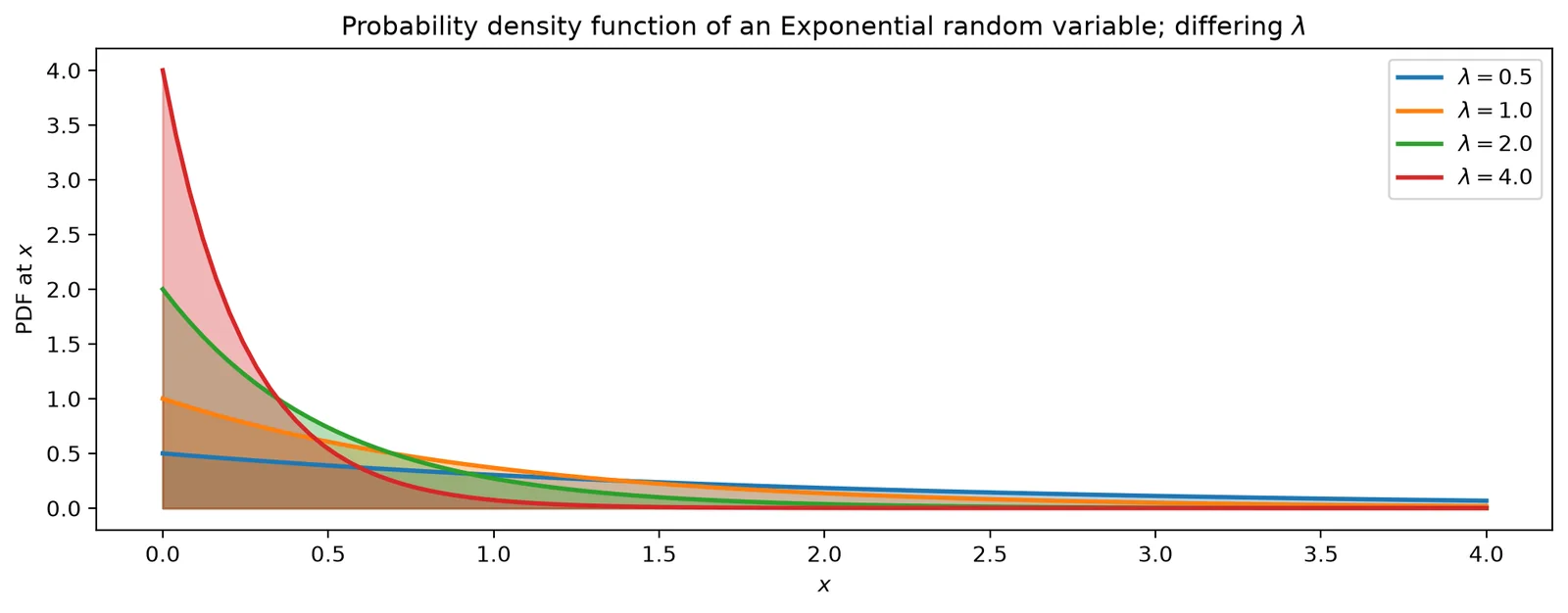
Exponential
The Exponantial probability function is
Therefore, the random variable X has an exponential distribution with parameter λ, we say X is exponential and write
Given a specific λ, the expected value of an exponential random variable is equal to the inverse of λ, that is:
_x = np.linspace(0, 4, 100)
expo = scipy.stats.expon
_lambda_ = [0.5, 1, 2, 4]
plt.figure(figsize=(12, 4))
for l, _c in zip(_lambda_, colors_1):
    plt.plot(_x, expo.pdf(_x, scale=1.0 / l), lw=2, color=_c, label='$\\lambda = %.1f$' % l)
    plt.fill_between(_x, expo.pdf(_x, scale=1.0 / l), color=_c, alpha=0.33)
plt.legend()
plt.ylabel('PDF at $x$')
plt.xlabel('$x$')
plt.title('Probability density function of an Exponential random variable; differing $\\lambda$')