Regression Analysis with Uncertainty
Regression analysis
def linreg(X, Y):
    """
    Summary
        Linear regression of y = ax + b
    Usage
        real, real, real = linreg(list, list)
    Returns coefficients to the regression line "y=ax+b" from x[] and y[], and R^2 Value
    """
    N = len(X)

    if N != len(Y):  raise(ValueError, 'unequal length')

    Sx = Sy = Sxx = Syy = Sxy = 0.0
    for x, y in zip(X, Y):
        Sx = Sx + x
        Sy = Sy + y
        Sxx = Sxx + x*x
        Syy = Syy + y*y
        Sxy = Sxy + x*y

    det =  Sx * Sx - Sxx * N # see the lecture

    a,b = (Sy * Sx - Sxy * N)/det, (Sx * Sxy - Sxx * Sy)/det

    meanerror = residual = residualx = 0.0

    for x, y in zip(X, Y):
        meanerror = meanerror + (y - Sy/N)**2
        residual = residual + (y - a * x - b)**2
        residualx = residualx + (x - Sx/N)**2

    RR = 1 - residual/meanerror
    # linear regression, a_0, a_1 => m = 1
    m = 1
    nu = N - (m+1)

    sxy = np.sqrt(residual / nu)

    # Var_a, Var_b = ss * N / det, ss * Sxx / det

    Sa = sxy * np.sqrt(1/residualx)
    Sb = sxy * np.sqrt(Sxx/(N*residualx))

    # We work with t-distribution, ()
    # t_{nu;\alpha/2} = t_{3,95} = 3.18
    tvalue = t.ppf(1-(1-0.95)/2, nu)

    print("Estimate: y = ax + b")
    print("N = %d" % N)
    print("Degrees of freedom $\\nu$ = %d " % nu)
    print("a = %.2f $\\pm$ %.3f" % (a, tvalue*Sa/np.sqrt(N)))
    print("b = %.2f $\\pm$ %.3f" % (b, tvalue*Sb/np.sqrt(N)))
    print("R^2 = %.3f" % RR)
    print("Syx = %.3f" % sxy)
    print("y = %.2f x + %.2f $\\pm$ %.3f V" % (a, b, tvalue*sxy/np.sqrt(N)))
    return a, b, RR, sxy
Linear potentiometer calibration: distance versus voltage
Estimate: y = ax + b
N = 5
Degrees of freedom $\nu$ = 3
a = 1.04 $\pm$ 0.072
b = 0.02 $\pm$ 0.238
R^2 = 0.993
Syx = 0.159
y = 1.04 x + 0.02 $\pm$ 0.227 V
fig,ax = plt.subplots(figsize=(8,8))
ax.plot(X,Y,'o')
ax.plot(X,(X*a + b),'r-')
ax.plot(X,(X*a + b +.23),'k--')
ax.plot(X,(X*a + b - .23),'k--')
ax.set_xlim((0,8))
ax.set_ylim((0,8))
ax.text(.5,4,'Range of $Y$')
ax.text(2,1,'Range of $X$')
ax.plot([0,1],[1,1],'k:')
ax.plot([0,5],[5.5,5.5],'k:')
ax.plot([1,1],[0,1],'k:')
ax.plot([5,5],[0,5.5],'k:')

ax.annotate('Confidence interval', xy=(4,4), xytext=(6,4),
            arrowprops=dict(facecolor='black', shrink=0.05,width=.1),
            )
ax.annotate('Confidence interval', xy=(4,4.5), xytext=(6,4),
            arrowprops=dict(facecolor='black', shrink=0.05,width=.1),
            )

ax.set_xlabel('$x$ (cm)',fontsize=16)
ax.set_ylabel('$y$ (V)',fontsize=16);
Example 2 - hot wire calibration
We expect the calibration from the King's law in the form:
\[ E = a + b U^m \]
U = np.array([0.0, 10.0, 20.0, 30.0, 40.0])
# given data:
E = np.array([3.19, 3.99, 4.3, 4.48, 4.65])  # air velocity, (m/s)  # voltage (V)
We want to use linear regression
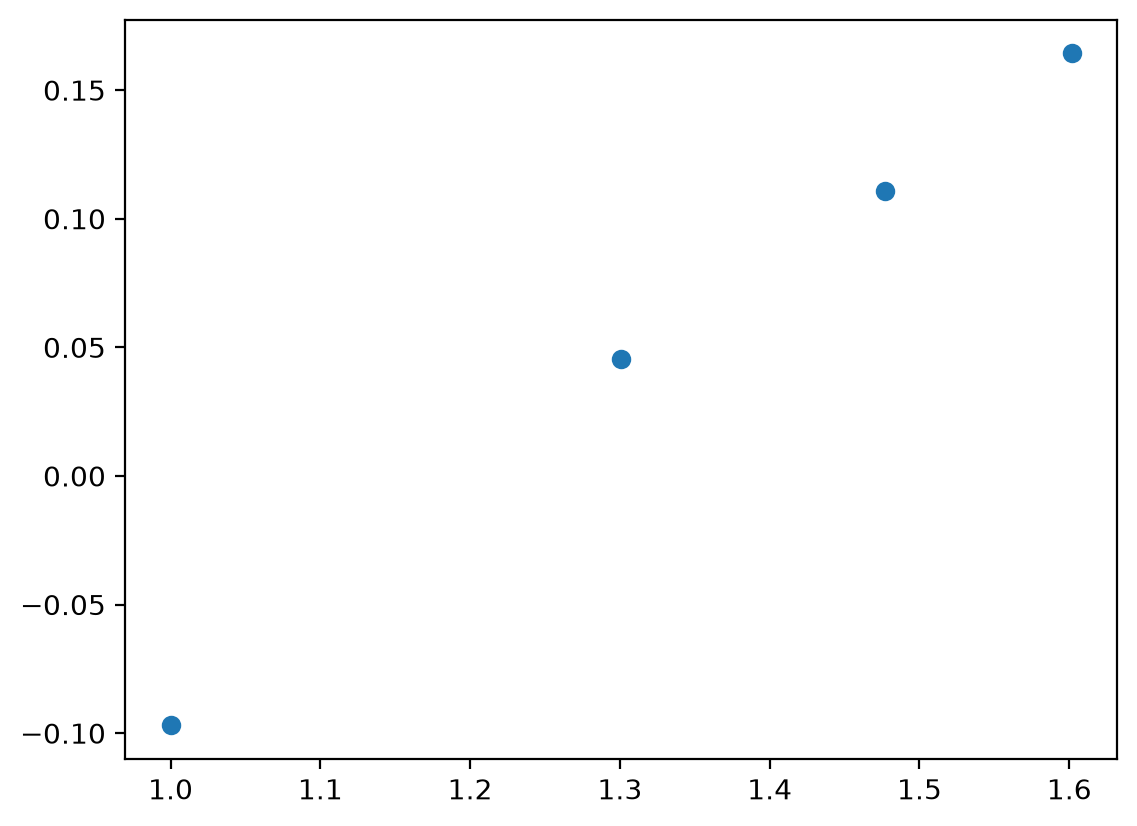
Therefore we convert it to linear form: $$ \log_{10}(E-a) = \log_{10} b + m\, \log_{10} U $$
and solve as linear regression:
\[ Y = B + m X \]
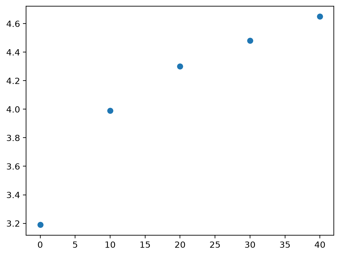
# since E(U = 0) = 3.19 V, we get a = 3.19 V
a_1 = 3.19  # V
plt.plot(np.log10(U[1:]), np.log10(E[1:] - a_1), 'o')
Estimate: y = ax + b
N = 4
Degrees of freedom $\nu$ = 2
a = 0.43 $\pm$ 0.033
b = -0.52 $\pm$ 0.045
R^2 = 0.997
Syx = 0.007
y = 0.43 x + -0.52 $\pm$ 0.015 V
\[ Y = -0.525 + 0.43 X \pm 0.015 (95\%) \]
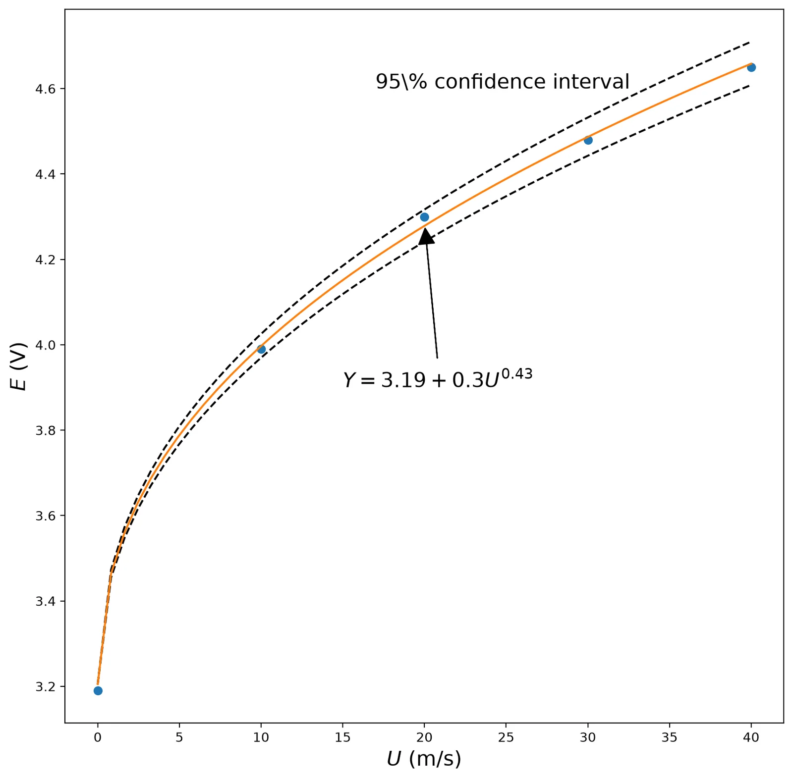
\[ E = 3.19 + 0.3 U^{0.43}\]
plt.figure(figsize=(10, 10))
plt.plot(U, E, 'o')
u = np.linspace(0.001, 40)
# for smooth plot
x = np.log10(u)
y = m * x + B
yu = y + 0.015
yl = y - 0.015
Es = 10 ** y + a_1  # linear confidence interval
Eu = 10 ** yu + a_1
El = 10 ** yl + a_1
plt.plot(u, El, 'k--')
plt.plot(u, Eu, 'k--')  # confidence interval non-linear
plt.plot(u, Es)
plt.xlabel('$U$ (m/s)', fontsize=16)
plt.ylabel('$E$ (V)', fontsize=16)
plt.text(17, 4.6, '95\\% confidence interval', fontsize=16)
plt.annotate('$Y = 3.19 + 0.3U^{0.43}$', xy=(20, 4.29), xytext=(15, 3.9), arrowprops=dict(facecolor='black', shrink=0.05, width=0.1), fontsize=16)