How to estimate the uncertainty of a slope for static calibration or regression
A calibration experiment gives you pairs of readings: you command an input U
and the instrument reports I. Plotting I against U should give a straight
line, and the slope of that line is the sensitivity of the instrument — the
number you actually want, with an uncertainty attached.
Here is one such series. We will do three things, in order:
- plot the measurements,
- attach error bars and fit a straight line,
- find the steepest and shallowest lines the data allow.
import matplotlib.pyplot as plt
import numpy as np

# Six calibration points: commanded voltage against reported current.
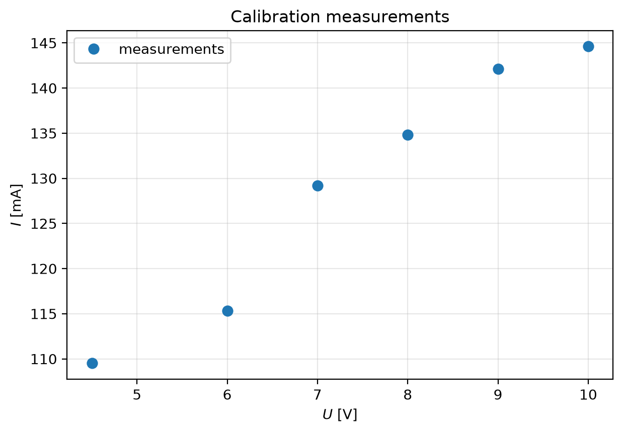
U = np.array([4.5, 6.0, 7.0, 8.0, 9.0, 10.0])  # voltage, V
I = np.array([109.5, 115.3, 129.2, 134.8, 142.1, 144.6])  # current, mA

du = 0.15  # standard uncertainty of the voltage reading, V
1. The measurements
Six points. There is a clear upward trend, but they do not lie exactly on a
line — that scatter is the measurement uncertainty we need to quantify.
fig1, ax1 = plt.subplots(figsize=(7, 4.5))
ax1.plot(U, I, "o", markersize=7, color="tab:blue", label="measurements")
ax1.set_xlabel("$U$ [V]")
ax1.set_ylabel("$I$ [mA]")
ax1.set_title("Calibration measurements")
ax1.grid(alpha=0.3)
ax1.legend()
fig1
2. Error bars and a least-squares fit
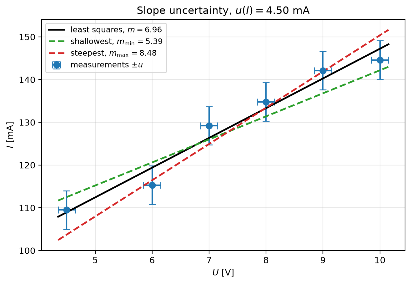
Each reading carries an uncertainty, drawn as an error bar. Drag the slider to
change the standard uncertainty u(I) of the current measurement and watch the
picture change.
np.polyfit(U, I, 1) returns the least-squares slope and intercept, which is
our best estimate \(m\).
m_best, intercept = np.polyfit(U, I, 1)
print(f"least-squares slope   m = {m_best:.2f} mA/V")
print(f"intercept                 = {intercept:.1f} mA")
least-squares slope   m = 6.96 mA/V
intercept                 = 77.6 mA
u_I = mo.ui.slider(
    start=1.0,
    stop=6.0,
    step=0.25,
    value=4.5,
    label="standard uncertainty of the current reading, u(I) [mA]",
)
u_I
3. The steepest and shallowest acceptable lines
Rather than trusting a formula, ask a geometric question: what is the range of
slopes for which some straight line still passes through every error bar?
The lines that just touch the error bars at one end give the two limits. Each
one ignores most of the points — that is the point. Only the pair of points
that binds the answer matters; the rest only have to be consistent.
def slope_limits(U, I, du, di):
    """Steepest and shallowest lines that cross every error bar.

    The line b + m*x crosses box i when it is above the bottom-right corner
    and below the top-left corner, i.e. for some b,

        (I_i - di) - m (U_i + du)  <=  b  <=  (I_i + di) - m (U_i - du)

    A b exists for all boxes only when every box is compatible with every
    other, which reduces to a bound on m per pair i, j:

        (I_i - di) - (I_j + di)  <=  m * [ (U_i + du) - (U_j - du) ]

    Taking the largest lower bound and the smallest upper bound over all
    pairs gives the interval of acceptable slopes. A box never constrains
    itself, so i == j is excluded.
    """
    n = len(U)
    i, j = np.meshgrid(np.arange(n), np.arange(n), indexing="ij")
    other = i != j
    gap = (U[i] + du) - (U[j] - du)
    rise = (I[i] - di) - (I[j] + di)
    safe = np.where(gap == 0, 1.0, gap)

    # gap > 0 forces m to be at least rise/gap; take the strongest such bound.
    m_lo = float(np.where(other & (gap > 0), rise / safe, -np.inf).max())
    # gap < 0 forces m to be at most rise/gap; take the strongest such bound.
    m_hi = float(np.where(other & (gap < 0), rise / safe, np.inf).min())

    feasible = m_lo <= m_hi
    return (m_lo, m_hi) if feasible else (np.nan, np.nan)

def touching_intercept(U, I, du, di, m):
    """Largest intercept for which the line of slope m still crosses every bar."""
    return float(np.max((I - di) - m * (U + du)))

m_min, m_max = slope_limits(U, I, du, u_I.value)
feasible = np.isfinite(m_min) and np.isfinite(m_max)

if feasible:
    b_min = touching_intercept(U, I, du, u_I.value, m_min)
    b_max = touching_intercept(U, I, du, u_I.value, m_max)
else:
    b_min = b_max = np.nan
fig2, ax2 = plt.subplots(figsize=(7.5, 4.8))
ax2.errorbar(
    U, I, xerr=du, yerr=u_I.value, fmt="o", markersize=7,
    capsize=4, color="tab:blue", label="measurements $\\pm u$",
)

if feasible:
    grid = np.linspace(U.min() - du, U.max() + du, 200)
    ax2.plot(grid, m_best * grid + intercept, "k-", lw=2,
            label=f"least squares, $m={m_best:.2f}$")
    ax2.plot(grid, m_min * grid + b_min, color="tab:green", ls="--", lw=2,
            label=f"shallowest, $m_{{\\min}}={m_min:.2f}$")
    ax2.plot(grid, m_max * grid + b_max, color="tab:red", ls="--", lw=2,
            label=f"steepest, $m_{{\\max}}={m_max:.2f}$")
else:
    ax2.plot([], [], " ")
    ax2.text(
        0.5, 0.06,
        "no single line crosses every error bar\nat this uncertainty",
        transform=ax2.transAxes, ha="center", va="bottom",
        color="tab:red", fontsize=11, weight="bold",
    )

ax2.set_xlabel("$U$ [V]")
ax2.set_ylabel("$I$ [mA]")
ax2.set_title(f"Slope uncertainty, $u(I)={u_I.value:.2f}$ mA")
ax2.grid(alpha=0.3)
ax2.legend(fontsize=9, loc="upper left")
fig2
if feasible:
    u_m = (m_max - m_min) / 2
    report = f"""
With $u(I) = {u_I.value:.2f}$ mA the acceptable slopes run from
$m_{{\\min}} = {m_min:.2f}$ to $m_{{\\max}} = {m_max:.2f}$ mA/V, so

$$\\Delta m = \\frac{{m_{{\\max}} - m_{{\\min}}}}{{2}} = {u_m:.2f}\\ \\text{{mA/V}}$$

and the slope is quoted as $m = {m_best:.1f} \\pm {u_m:.1f}$ mA/V.

Shrink the slider: below about 2.2 mA **no** straight line passes through every
error bar, which is the method correctly telling you that the uncertainty you
claimed is too small to explain your own scatter.
"""
else:
    report = f"""
At $u(I) = {u_I.value:.2f}$ mA there is **no** straight line that passes through
every error bar — the points are more scattered than the quoted uncertainty
allows, so the slope is not bracketed at all. Widen the error bars until a line
fits.
"""
mo.md(report)
With \(u(I) = 4.50\) mA the acceptable slopes run from
\(m_{\min} = 5.39\) to \(m_{\max} = 8.48\) mA/V, so
\[\Delta m = \frac{m_{\max} - m_{\min}}{2} = 1.54\ \text{mA/V}\]
and the slope is quoted as \(m = 7.0 \pm 1.5\) mA/V.
Shrink the slider: below about 2.2 mA no straight line passes through every
error bar, which is the method correctly telling you that the uncertainty you
claimed is too small to explain your own scatter.
Where the bound comes from
Write the candidate line as \(I = b + m\,U\). Reading \(I\) at \(U\) means
interpolating within a rectangle of half-widths \(d_U\) in voltage and \(d_I\) in
current. The line enters the rectangle at its left edge and leaves at its
right edge, so it crosses that rectangle exactly when
\[
I_i - d_I \;\le\; b + m\,(U_i + d_U)
\qquad\text{and}\qquad
b + m\,(U_i - d_U) \;\le\; I_i + d_I ,
\]
that is, when some intercept \(b\) satisfies
\[
(I_i - d_I) - m\,(U_i + d_U) \;\le\; b \;\le\; (I_i + d_I) - m\,(U_i - d_U).
\]
A single line must satisfy this for every point at once, so the best any
intercept can do must sit above every lower bound and below every upper bound.
Pairing a lower bound from point \(i\) with an upper bound from point \(j\) gives
\[
(I_i - d_I) - (I_j + d_I) \;\le\; m\,\big[(U_i + d_U) - (U_j - d_U)\big].
\]
When the bracket is positive this is a lower bound on the slope; when it is
negative it is an upper bound. Collecting every pair and keeping the
strongest of each kind,
\[
m_{\min} = \max_{i \ne j} \frac{(I_i - d_I) - (I_j + d_I)}{(U_i + d_U) - (U_j - d_U)},
\qquad
m_{\max} = \min_{i \ne j} \frac{(I_i - d_I) - (I_j + d_I)}{(U_i + d_U) - (U_j - d_U)}
\]
over the pairs where the denominator has the required sign. A pair \(i = j\) is
excluded, since a box never constrains itself.
Note which points survive. Only the pair that produces the largest lower bound
actually sets \(m_{\min}\), and only the pair producing the smallest upper bound
sets \(m_{\max}\) — every other point merely has to stay consistent. That is
the "ignore some of the points" step: the extreme slopes are pinned down by two
readings, not by a fit to all six.
Reporting
The interval is not a statistical confidence interval, so it is quoted as a
half-width rather than as a standard uncertainty, and with the correct number
of significant figures:
\[
m = m_{\text{best}} \pm \frac{m_{\max} - m_{\min}}{2},
\]
both terms rounded to the same decimal place — \(7.3 \pm 1.9\) mA/V, not
\(7.28 \pm 1.874\) mA/V.
Two cautions
- This construction assumes a single line really is the right model. If the
scatter is curved rather than random, no line will cross every error bar
at any width, and you have found a hysteresis or a nonlinearity instead of
an uncertainty.
- The bound widens as the error bars grow, so quoting an uncertainty makes the
method agree with it. Judge it against a second, independent method — a
weighted least-squares fit with its own residual estimate, or a Monte Carlo
propagation.
{"var_name":"u_I","kind":"slider","values":[1,1.25,1.5,1.75,2,2.25,2.5,2.75,3,3.25,3.5,3.75,4,4.25,4.5,4.75,5,5.25,5.5,5.75,6],"default":4.5,"label":"standard uncertainty of the current reading, u(I) [mA]"}
{"1":{"8":"\u003cdiv class=\"language-python highlight\"\u003e\u003cpre\u003e\u003cspan\u003e\u003c/span\u003e\u003ccode\u003e\u003cspan id=\"__span-0-1\"\u003e\u003ca id=\"__codelineno-0-1\" name=\"__codelineno-0-1\" href=\"#__codelineno-0-1\"\u003e\u003c/a\u003e\u003cspan class=\"n\"\u003eu_I\u003c/span\u003e \u003cspan class=\"o\"\u003e=\u003c/span\u003e \u003cspan class=\"n\"\u003emo\u003c/span\u003e\u003cspan class=\"o\"\u003e.\u003c/span\u003e\u003cspan class=\"n\"\u003eui\u003c/span\u003e\u003cspan class=\"o\"\u003e.\u003c/span\u003e\u003cspan class=\"n\"\u003eslider\u003c/span\u003e\u003cspan class=\"p\"\u003e(\u003c/span\u003e\u003cspan class=\"n\"\u003estart\u003c/span\u003e\u003cspan class=\"o\"\u003e=\u003c/span\u003e\u003cspan class=\"mf\"\u003e1.0\u003c/span\u003e\u003cspan class=\"p\"\u003e,\u003c/span\u003e \u003cspan class=\"n\"\u003estop\u003c/span\u003e\u003cspan class=\"o\"\u003e=\u003c/span\u003e\u003cspan class=\"mf\"\u003e6.0\u003c/span\u003e\u003cspan class=\"p\"\u003e,\u003c/span\u003e \u003cspan class=\"n\"\u003estep\u003c/span\u003e\u003cspan class=\"o\"\u003e=\u003c/span\u003e\u003cspan class=\"mf\"\u003e0.25\u003c/span\u003e\u003cspan class=\"p\"\u003e,\u003c/span\u003e \u003cspan class=\"n\"\u003evalue\u003c/span\u003e\u003cspan class=\"o\"\u003e=\u003c/span\u003e\u003cspan class=\"mi\"\u003e1\u003c/span\u003e\u003cspan class=\"p\"\u003e,\u003c/span\u003e \u003cspan class=\"n\"\u003elabel\u003c/span\u003e\u003cspan class=\"o\"\u003e=\u003c/span\u003e\u003cspan class=\"s1\"\u003e'standard uncertainty of the current reading, u(I) [mA]'\u003c/span\u003e\u003cspan class=\"p\"\u003e)\u003c/span\u003e\n\u003c/span\u003e\u003cspan id=\"__span-0-2\"\u003e\u003ca id=\"__codelineno-0-2\" name=\"__codelineno-0-2\" href=\"#__codelineno-0-2\"\u003e\u003c/a\u003e\u003cspan class=\"n\"\u003eu_I\u003c/span\u003e\n\u003c/span\u003e\u003c/code\u003e\u003c/pre\u003e\u003c/div\u003e\n\u003cdiv class=\"marimo-book-output\"\u003e\n\u003cmarimo-slider data-initial-value='1' data-label='\u0026quot;\u0026#92;u003cspan class=\u0026#92;\u0026quot;markdown prose dark:prose-invert contents\u0026#92;\u0026quot;\u0026#92;u003e\u0026#92;u003cspan class=\u0026#92;\u0026quot;paragraph\u0026#92;\u0026quot;\u0026#92;u003estandard uncertainty of the current reading, u(I) [mA]\u0026#92;u003c/span\u0026#92;u003e\u0026#92;u003c/span\u0026#92;u003e\u0026quot;' data-start='1.0' data-stop='6.0' data-step='0.25' data-steps='[]' data-debounce='false' data-disabled='false' data-orientation='\u0026quot;horizontal\u0026quot;' data-show-value='false' data-include-input='false' data-full-width='false'\u003e\u003c/marimo-slider\u003e\n\u003c/div\u003e","11":"\u003cdiv class=\"language-python highlight\"\u003e\u003cpre\u003e\u003cspan\u003e\u003c/span\u003e\u003ccode\u003e\u003cspan id=\"__span-0-1\"\u003e\u003ca id=\"__codelineno-0-1\" name=\"__codelineno-0-1\" href=\"#__codelineno-0-1\"\u003e\u003c/a\u003e\u003cspan class=\"n\"\u003efig2\u003c/span\u003e\u003cspan class=\"p\"\u003e,\u003c/span\u003e \u003cspan class=\"n\"\u003eax2\u003c/span\u003e \u003cspan class=\"o\"\u003e=\u003c/span\u003e \u003cspan class=\"n\"\u003eplt\u003c/span\u003e\u003cspan class=\"o\"\u003e.\u003c/span\u003e\u003cspan class=\"n\"\u003esubplots\u003c/span\u003e\u003cspan class=\"p\"\u003e(\u003c/span\u003e\u003cspan class=\"n\"\u003efigsize\u003c/span\u003e\u003cspan class=\"o\"\u003e=\u003c/span\u003e\u003cspan class=\"p\"\u003e(\u003c/span\u003e\u003cspan class=\"mf\"\u003e7.5\u003c/span\u003e\u003cspan class=\"p\"\u003e,\u003c/span\u003e \u003cspan class=\"mf\"\u003e4.8\u003c/span\u003e\u003cspan class=\"p\"\u003e))\u003c/span\u003e\n\u003c/span\u003e\u003cspan id=\"__span-0-2\"\u003e\u003ca id=\"__codelineno-0-2\" name=\"__codelineno-0-2\" href=\"#__codelineno-0-2\"\u003e\u003c/a\u003e\u003cspan class=\"n\"\u003eax2\u003c/span\u003e\u003cspan class=\"o\"\u003e.\u003c/span\u003e\u003cspan class=\"n\"\u003eerrorbar\u003c/span\u003e\u003cspan class=\"p\"\u003e(\u003c/span\u003e\n\u003c/span\u003e\u003cspan id=\"__span-0-3\"\u003e\u003ca id=\"__codelineno-0-3\" name=\"__codelineno-0-3\" href=\"#__codelineno-0-3\"\u003e\u003c/a\u003e \u003cspan class=\"n\"\u003eU\u003c/span\u003e\u003cspan class=\"p\"\u003e,\u003c/span\u003e \u003cspan class=\"n\"\u003eI\u003c/span\u003e\u003cspan class=\"p\"\u003e,\u003c/span\u003e \u003cspan class=\"n\"\u003exerr\u003c/span\u003e\u003cspan class=\"o\"\u003e=\u003c/span\u003e\u003cspan class=\"n\"\u003edu\u003c/span\u003e\u003cspan class=\"p\"\u003e,\u003c/span\u003e \u003cspan class=\"n\"\u003eyerr\u003c/span\u003e\u003cspan class=\"o\"\u003e=\u003c/span\u003e\u003cspan class=\"n\"\u003eu_I\u003c/span\u003e\u003cspan class=\"o\"\u003e.\u003c/span\u003e\u003cspan class=\"n\"\u003evalue\u003c/span\u003e\u003cspan class=\"p\"\u003e,\u003c/span\u003e \u003cspan class=\"n\"\u003efmt\u003c/span\u003e\u003cspan class=\"o\"\u003e=\u003c/span\u003e\u003cspan class=\"s2\"\u003e\"o\"\u003c/span\u003e\u003cspan class=\"p\"\u003e,\u003c/span\u003e \u003cspan class=\"n\"\u003emarkersize\u003c/span\u003e\u003cspan class=\"o\"\u003e=\u003c/span\u003e\u003cspan class=\"mi\"\u003e7\u003c/span\u003e\u003cspan class=\"p\"\u003e,\u003c/span\u003e\n\u003c/span\u003e\u003cspan id=\"__span-0-4\"\u003e\u003ca id=\"__codelineno-0-4\" name=\"__codelineno-0-4\" href=\"#__codelineno-0-4\"\u003e\u003c/a\u003e \u003cspan class=\"n\"\u003ecapsize\u003c/span\u003e\u003cspan class=\"o\"\u003e=\u003c/span\u003e\u003cspan class=\"mi\"\u003e4\u003c/span\u003e\u003cspan class=\"p\"\u003e,\u003c/span\u003e \u003cspan class=\"n\"\u003ecolor\u003c/span\u003e\u003cspan class=\"o\"\u003e=\u003c/span\u003e\u003cspan class=\"s2\"\u003e\"tab:blue\"\u003c/span\u003e\u003cspan class=\"p\"\u003e,\u003c/span\u003e \u003cspan class=\"n\"\u003elabel\u003c/span\u003e\u003cspan class=\"o\"\u003e=\u003c/span\u003e\u003cspan class=\"s2\"\u003e\"measurements $\u003c/span\u003e\u003cspan class=\"se\"\u003e\\\\\u003c/span\u003e\u003cspan class=\"s2\"\u003epm u$\"\u003c/span\u003e\u003cspan class=\"p\"\u003e,\u003c/span\u003e\n\u003c/span\u003e\u003cspan id=\"__span-0-5\"\u003e\u003ca id=\"__codelineno-0-5\" name=\"__codelineno-0-5\" href=\"#__codelineno-0-5\"\u003e\u003c/a\u003e\u003cspan class=\"p\"\u003e)\u003c/span\u003e\n\u003c/span\u003e\u003cspan id=\"__span-0-6\"\u003e\u003ca id=\"__codelineno-0-6\" name=\"__codelineno-0-6\" href=\"#__codelineno-0-6\"\u003e\u003c/a\u003e\n\u003c/span\u003e\u003cspan id=\"__span-0-7\"\u003e\u003ca id=\"__codelineno-0-7\" name=\"__codelineno-0-7\" href=\"#__codelineno-0-7\"\u003e\u003c/a\u003e\u003cspan class=\"k\"\u003eif\u003c/span\u003e \u003cspan class=\"n\"\u003efeasible\u003c/span\u003e\u003cspan class=\"p\"\u003e:\u003c/span\u003e\n\u003c/span\u003e\u003cspan id=\"__span-0-8\"\u003e\u003ca id=\"__codelineno-0-8\" name=\"__codelineno-0-8\" href=\"#__codelineno-0-8\"\u003e\u003c/a\u003e \u003cspan class=\"n\"\u003egrid\u003c/span\u003e \u003cspan class=\"o\"\u003e=\u003c/span\u003e \u003cspan class=\"n\"\u003enp\u003c/span\u003e\u003cspan class=\"o\"\u003e.\u003c/span\u003e\u003cspan class=\"n\"\u003elinspace\u003c/span\u003e\u003cspan class=\"p\"\u003e(\u003c/span\u003e\u003cspan class=\"n\"\u003eU\u003c/span\u003e\u003cspan class=\"o\"\u003e.\u003c/span\u003e\u003cspan class=\"n\"\u003emin\u003c/span\u003e\u003cspan class=\"p\"\u003e()\u003c/span\u003e \u003cspan class=\"o\"\u003e-\u003c/span\u003e \u003cspan class=\"n\"\u003edu\u003c/span\u003e\u003cspan class=\"p\"\u003e,\u003c/span\u003e \u003cspan class=\"n\"\u003eU\u003c/span\u003e\u003cspan class=\"o\"\u003e.\u003c/span\u003e\u003cspan class=\"n\"\u003emax\u003c/span\u003e\u003cspan class=\"p\"\u003e()\u003c/span\u003e \u003cspan class=\"o\"\u003e+\u003c/span\u003e \u003cspan class=\"n\"\u003edu\u003c/span\u003e\u003cspan class=\"p\"\u003e,\u003c/span\u003e \u003cspan class=\"mi\"\u003e200\u003c/span\u003e\u003cspan class=\"p\"\u003e)\u003c/span\u003e\n\u003c/span\u003e\u003cspan id=\"__span-0-9\"\u003e\u003ca id=\"__codelineno-0-9\" name=\"__codelineno-0-9\" href=\"#__codelineno-0-9\"\u003e\u003c/a\u003e \u003cspan class=\"n\"\u003eax2\u003c/span\u003e\u003cspan class=\"o\"\u003e.\u003c/span\u003e\u003cspan class=\"n\"\u003eplot\u003c/span\u003e\u003cspan class=\"p\"\u003e(\u003c/span\u003e\u003cspan class=\"n\"\u003egrid\u003c/span\u003e\u003cspan class=\"p\"\u003e,\u003c/span\u003e \u003cspan class=\"n\"\u003em_best\u003c/span\u003e \u003cspan class=\"o\"\u003e*\u003c/span\u003e \u003cspan class=\"n\"\u003egrid\u003c/span\u003e \u003cspan class=\"o\"\u003e+\u003c/span\u003e \u003cspan class=\"n\"\u003eintercept\u003c/span\u003e\u003cspan class=\"p\"\u003e,\u003c/span\u003e \u003cspan class=\"s2\"\u003e\"k-\"\u003c/span\u003e\u003cspan class=\"p\"\u003e,\u003c/span\u003e \u003cspan class=\"n\"\u003elw\u003c/span\u003e\u003cspan class=\"o\"\u003e=\u003c/span\u003e\u003cspan class=\"mi\"\u003e2\u003c/span\u003e\u003cspan class=\"p\"\u003e,\u003c/span\u003e\n\u003c/span\u003e\u003cspan id=\"__span-0-10\"\u003e\u003ca id=\"__codelineno-0-10\" name=\"__codelineno-0-10\" href=\"#__codelineno-0-10\"\u003e\u003c/a\u003e \u003cspan class=\"n\"\u003elabel\u003c/span\u003e\u003cspan class=\"o\"\u003e=\u003c/span\u003e\u003cspan class=\"sa\"\u003ef\u003c/span\u003e\u003cspan class=\"s2\"\u003e\"least squares, $m=\u003c/span\u003e\u003cspan class=\"si\"\u003e{\u003c/span\u003e\u003cspan class=\"n\"\u003em_best\u003c/span\u003e\u003cspan class=\"si\"\u003e:\u003c/span\u003e\u003cspan class=\"s2\"\u003e.2f\u003c/span\u003e\u003cspan class=\"si\"\u003e}\u003c/span\u003e\u003cspan class=\"s2\"\u003e$\"\u003c/span\u003e\u003cspan class=\"p\"\u003e)\u003c/span\u003e\n\u003c/span\u003e\u003cspan id=\"__span-0-11\"\u003e\u003ca id=\"__codelineno-0-11\" name=\"__codelineno-0-11\" href=\"#__codelineno-0-11\"\u003e\u003c/a\u003e \u003cspan class=\"n\"\u003eax2\u003c/span\u003e\u003cspan class=\"o\"\u003e.\u003c/span\u003e\u003cspan class=\"n\"\u003eplot\u003c/span\u003e\u003cspan class=\"p\"\u003e(\u003c/span\u003e\u003cspan class=\"n\"\u003egrid\u003c/span\u003e\u003cspan class=\"p\"\u003e,\u003c/span\u003e \u003cspan class=\"n\"\u003em_min\u003c/span\u003e \u003cspan class=\"o\"\u003e*\u003c/span\u003e \u003cspan class=\"n\"\u003egrid\u003c/span\u003e \u003cspan class=\"o\"\u003e+\u003c/span\u003e \u003cspan class=\"n\"\u003eb_min\u003c/span\u003e\u003cspan class=\"p\"\u003e,\u003c/span\u003e \u003cspan class=\"n\"\u003ecolor\u003c/span\u003e\u003cspan class=\"o\"\u003e=\u003c/span\u003e\u003cspan class=\"s2\"\u003e\"tab:green\"\u003c/span\u003e\u003cspan class=\"p\"\u003e,\u003c/span\u003e \u003cspan class=\"n\"\u003els\u003c/span\u003e\u003cspan class=\"o\"\u003e=\u003c/span\u003e\u003cspan class=\"s2\"\u003e\"--\"\u003c/span\u003e\u003cspan class=\"p\"\u003e,\u003c/span\u003e \u003cspan class=\"n\"\u003elw\u003c/span\u003e\u003cspan class=\"o\"\u003e=\u003c/span\u003e\u003cspan class=\"mi\"\u003e2\u003c/span\u003e\u003cspan class=\"p\"\u003e,\u003c/span\u003e\n\u003c/span\u003e\u003cspan id=\"__span-0-12\"\u003e\u003ca id=\"__codelineno-0-12\" name=\"__codelineno-0-12\" href=\"#__codelineno-0-12\"\u003e\u003c/a\u003e \u003cspan class=\"n\"\u003elabel\u003c/span\u003e\u003cspan class=\"o\"\u003e=\u003c/span\u003e\u003cspan class=\"sa\"\u003ef\u003c/span\u003e\u003cspan class=\"s2\"\u003e\"shallowest, $m_\u003c/span\u003e\u003cspan class=\"se\"\u003e{{\\\\\u003c/span\u003e\u003cspan class=\"s2\"\u003emin\u003c/span\u003e\u003cspan class=\"se\"\u003e}}\u003c/span\u003e\u003cspan class=\"s2\"\u003e=\u003c/span\u003e\u003cspan class=\"si\"\u003e{\u003c/span\u003e\u003cspan class=\"n\"\u003em_min\u003c/span\u003e\u003cspan class=\"si\"\u003e:\u003c/span\u003e\u003cspan class=\"s2\"\u003e.2f\u003c/span\u003e\u003cspan class=\"si\"\u003e}\u003c/span\u003e\u003cspan class=\"s2\"\u003e$\"\u003c/span\u003e\u003cspan class=\"p\"\u003e)\u003c/span\u003e\n\u003c/span\u003e\u003cspan id=\"__span-0-13\"\u003e\u003ca id=\"__codelineno-0-13\" name=\"__codelineno-0-13\" href=\"#__codelineno-0-13\"\u003e\u003c/a\u003e \u003cspan class=\"n\"\u003eax2\u003c/span\u003e\u003cspan class=\"o\"\u003e.\u003c/span\u003e\u003cspan class=\"n\"\u003eplot\u003c/span\u003e\u003cspan class=\"p\"\u003e(\u003c/span\u003e\u003cspan class=\"n\"\u003egrid\u003c/span\u003e\u003cspan class=\"p\"\u003e,\u003c/span\u003e \u003cspan class=\"n\"\u003em_max\u003c/span\u003e \u003cspan class=\"o\"\u003e*\u003c/span\u003e \u003cspan class=\"n\"\u003egrid\u003c/span\u003e \u003cspan class=\"o\"\u003e+\u003c/span\u003e \u003cspan class=\"n\"\u003eb_max\u003c/span\u003e\u003cspan class=\"p\"\u003e,\u003c/span\u003e \u003cspan class=\"n\"\u003ecolor\u003c/span\u003e\u003cspan class=\"o\"\u003e=\u003c/span\u003e\u003cspan class=\"s2\"\u003e\"tab:red\"\u003c/span\u003e\u003cspan class=\"p\"\u003e,\u003c/span\u003e \u003cspan class=\"n\"\u003els\u003c/span\u003e\u003cspan class=\"o\"\u003e=\u003c/span\u003e\u003cspan class=\"s2\"\u003e\"--\"\u003c/span\u003e\u003cspan class=\"p\"\u003e,\u003c/span\u003e \u003cspan class=\"n\"\u003elw\u003c/span\u003e\u003cspan class=\"o\"\u003e=\u003c/span\u003e\u003cspan class=\"mi\"\u003e2\u003c/span\u003e\u003cspan class=\"p\"\u003e,\u003c/span\u003e\n\u003c/span\u003e\u003cspan id=\"__span-0-14\"\u003e\u003ca id=\"__codelineno-0-14\" name=\"__codelineno-0-14\" href=\"#__codelineno-0-14\"\u003e\u003c/a\u003e \u003cspan class=\"n\"\u003elabel\u003c/span\u003e\u003cspan class=\"o\"\u003e=\u003c/span\u003e\u003cspan class=\"sa\"\u003ef\u003c/span\u003e\u003cspan class=\"s2\"\u003e\"steepest, $m_\u003c/span\u003e\u003cspan class=\"se\"\u003e{{\\\\\u003c/span\u003e\u003cspan class=\"s2\"\u003emax\u003c/span\u003e\u003cspan class=\"se\"\u003e}}\u003c/span\u003e\u003cspan class=\"s2\"\u003e=\u003c/span\u003e\u003cspan class=\"si\"\u003e{\u003c/span\u003e\u003cspan class=\"n\"\u003em_max\u003c/span\u003e\u003cspan class=\"si\"\u003e:\u003c/span\u003e\u003cspan class=\"s2\"\u003e.2f\u003c/span\u003e\u003cspan class=\"si\"\u003e}\u003c/span\u003e\u003cspan class=\"s2\"\u003e$\"\u003c/span\u003e\u003cspan class=\"p\"\u003e)\u003c/span\u003e\n\u003c/span\u003e\u003cspan id=\"__span-0-15\"\u003e\u003ca id=\"__codelineno-0-15\" name=\"__codelineno-0-15\" href=\"#__codelineno-0-15\"\u003e\u003c/a\u003e\u003cspan class=\"k\"\u003eelse\u003c/span\u003e\u003cspan class=\"p\"\u003e:\u003c/span\u003e\n\u003c/span\u003e\u003cspan id=\"__span-0-16\"\u003e\u003ca id=\"__codelineno-0-16\" name=\"__codelineno-0-16\" href=\"#__codelineno-0-16\"\u003e\u003c/a\u003e \u003cspan class=\"n\"\u003eax2\u003c/span\u003e\u003cspan class=\"o\"\u003e.\u003c/span\u003e\u003cspan class=\"n\"\u003eplot\u003c/span\u003e\u003cspan class=\"p\"\u003e([],\u003c/span\u003e \u003cspan class=\"p\"\u003e[],\u003c/span\u003e \u003cspan class=\"s2\"\u003e\" \"\u003c/span\u003e\u003cspan class=\"p\"\u003e)\u003c/span\u003e\n\u003c/span\u003e\u003cspan id=\"__span-0-17\"\u003e\u003ca id=\"__codelineno-0-17\" name=\"__codelineno-0-17\" href=\"#__codelineno-0-17\"\u003e\u003c/a\u003e \u003cspan class=\"n\"\u003eax2\u003c/span\u003e\u003cspan class=\"o\"\u003e.\u003c/span\u003e\u003cspan class=\"n\"\u003etext\u003c/span\u003e\u003cspan class=\"p\"\u003e(\u003c/span\u003e\n\u003c/span\u003e\u003cspan id=\"__span-0-18\"\u003e\u003ca id=\"__codelineno-0-18\" name=\"__codelineno-0-18\" href=\"#__codelineno-0-18\"\u003e\u003c/a\u003e \u003cspan class=\"mf\"\u003e0.5\u003c/span\u003e\u003cspan class=\"p\"\u003e,\u003c/span\u003e \u003cspan class=\"mf\"\u003e0.06\u003c/span\u003e\u003cspan class=\"p\"\u003e,\u003c/span\u003e\n\u003c/span\u003e\u003cspan id=\"__span-0-19\"\u003e\u003ca id=\"__codelineno-0-19\" name=\"__codelineno-0-19\" href=\"#__codelineno-0-19\"\u003e\u003c/a\u003e \u003cspan class=\"s2\"\u003e\"no single line crosses every error bar\u003c/span\u003e\u003cspan class=\"se\"\u003e\\n\u003c/span\u003e\u003cspan class=\"s2\"\u003eat this uncertainty\"\u003c/span\u003e\u003cspan class=\"p\"\u003e,\u003c/span\u003e\n\u003c/span\u003e\u003cspan id=\"__span-0-20\"\u003e\u003ca id=\"__codelineno-0-20\" name=\"__codelineno-0-20\" href=\"#__codelineno-0-20\"\u003e\u003c/a\u003e \u003cspan class=\"n\"\u003etransform\u003c/span\u003e\u003cspan class=\"o\"\u003e=\u003c/span\u003e\u003cspan class=\"n\"\u003eax2\u003c/span\u003e\u003cspan class=\"o\"\u003e.\u003c/span\u003e\u003cspan class=\"n\"\u003etransAxes\u003c/span\u003e\u003cspan class=\"p\"\u003e,\u003c/span\u003e \u003cspan class=\"n\"\u003eha\u003c/span\u003e\u003cspan class=\"o\"\u003e=\u003c/span\u003e\u003cspan class=\"s2\"\u003e\"center\"\u003c/span\u003e\u003cspan class=\"p\"\u003e,\u003c/span\u003e \u003cspan class=\"n\"\u003eva\u003c/span\u003e\u003cspan class=\"o\"\u003e=\u003c/span\u003e\u003cspan class=\"s2\"\u003e\"bottom\"\u003c/span\u003e\u003cspan class=\"p\"\u003e,\u003c/span\u003e\n\u003c/span\u003e\u003cspan id=\"__span-0-21\"\u003e\u003ca id=\"__codelineno-0-21\" name=\"__codelineno-0-21\" href=\"#__codelineno-0-21\"\u003e\u003c/a\u003e \u003cspan class=\"n\"\u003ecolor\u003c/span\u003e\u003cspan class=\"o\"\u003e=\u003c/span\u003e\u003cspan class=\"s2\"\u003e\"tab:red\"\u003c/span\u003e\u003cspan class=\"p\"\u003e,\u003c/span\u003e \u003cspan class=\"n\"\u003efontsize\u003c/span\u003e\u003cspan class=\"o\"\u003e=\u003c/span\u003e\u003cspan class=\"mi\"\u003e11\u003c/span\u003e\u003cspan class=\"p\"\u003e,\u003c/span\u003e \u003cspan class=\"n\"\u003eweight\u003c/span\u003e\u003cspan class=\"o\"\u003e=\u003c/span\u003e\u003cspan class=\"s2\"\u003e\"bold\"\u003c/span\u003e\u003cspan class=\"p\"\u003e,\u003c/span\u003e\n\u003c/span\u003e\u003cspan id=\"__span-0-22\"\u003e\u003ca id=\"__codelineno-0-22\" name=\"__codelineno-0-22\" href=\"#__codelineno-0-22\"\u003e\u003c/a\u003e \u003cspan class=\"p\"\u003e)\u003c/span\u003e\n\u003c/span\u003e\u003cspan id=\"__span-0-23\"\u003e\u003ca id=\"__codelineno-0-23\" name=\"__codelineno-0-23\" href=\"#__codelineno-0-23\"\u003e\u003c/a\u003e\n\u003c/span\u003e\u003cspan id=\"__span-0-24\"\u003e\u003ca id=\"__codelineno-0-24\" name=\"__codelineno-0-24\" href=\"#__codelineno-0-24\"\u003e\u003c/a\u003e\u003cspan class=\"n\"\u003eax2\u003c/span\u003e\u003cspan class=\"o\"\u003e.\u003c/span\u003e\u003cspan class=\"n\"\u003eset_xlabel\u003c/span\u003e\u003cspan class=\"p\"\u003e(\u003c/span\u003e\u003cspan class=\"s2\"\u003e\"$U$ [V]\"\u003c/span\u003e\u003cspan class=\"p\"\u003e)\u003c/span\u003e\n\u003c/span\u003e\u003cspan id=\"__span-0-25\"\u003e\u003ca id=\"__codelineno-0-25\" name=\"__codelineno-0-25\" href=\"#__codelineno-0-25\"\u003e\u003c/a\u003e\u003cspan class=\"n\"\u003eax2\u003c/span\u003e\u003cspan class=\"o\"\u003e.\u003c/span\u003e\u003cspan class=\"n\"\u003eset_ylabel\u003c/span\u003e\u003cspan class=\"p\"\u003e(\u003c/span\u003e\u003cspan class=\"s2\"\u003e\"$I$ [mA]\"\u003c/span\u003e\u003cspan class=\"p\"\u003e)\u003c/span\u003e\n\u003c/span\u003e\u003cspan id=\"__span-0-26\"\u003e\u003ca id=\"__codelineno-0-26\" name=\"__codelineno-0-26\" href=\"#__codelineno-0-26\"\u003e\u003c/a\u003e\u003cspan class=\"n\"\u003eax2\u003c/span\u003e\u003cspan class=\"o\"\u003e.\u003c/span\u003e\u003cspan class=\"n\"\u003eset_title\u003c/span\u003e\u003cspan class=\"p\"\u003e(\u003c/span\u003e\u003cspan class=\"sa\"\u003ef\u003c/span\u003e\u003cspan class=\"s2\"\u003e\"Slope uncertainty, $u(I)=\u003c/span\u003e\u003cspan class=\"si\"\u003e{\u003c/span\u003e\u003cspan class=\"n\"\u003eu_I\u003c/span\u003e\u003cspan class=\"o\"\u003e.\u003c/span\u003e\u003cspan class=\"n\"\u003evalue\u003c/span\u003e\u003cspan class=\"si\"\u003e:\u003c/span\u003e\u003cspan class=\"s2\"\u003e.2f\u003c/span\u003e\u003cspan class=\"si\"\u003e}\u003c/span\u003e\u003cspan class=\"s2\"\u003e$ mA\"\u003c/span\u003e\u003cspan class=\"p\"\u003e)\u003c/span\u003e\n\u003c/span\u003e\u003cspan id=\"__span-0-27\"\u003e\u003ca id=\"__codelineno-0-27\" name=\"__codelineno-0-27\" href=\"#__codelineno-0-27\"\u003e\u003c/a\u003e\u003cspan class=\"n\"\u003eax2\u003c/span\u003e\u003cspan class=\"o\"\u003e.\u003c/span\u003e\u003cspan class=\"n\"\u003egrid\u003c/span\u003e\u003cspan class=\"p\"\u003e(\u003c/span\u003e\u003cspan class=\"n\"\u003ealpha\u003c/span\u003e\u003cspan class=\"o\"\u003e=\u003c/span\u003e\u003cspan class=\"mf\"\u003e0.3\u003c/span\u003e\u003cspan class=\"p\"\u003e)\u003c/span\u003e\n\u003c/span\u003e\u003cspan id=\"__span-0-28\"\u003e\u003ca id=\"__codelineno-0-28\" name=\"__codelineno-0-28\" href=\"#__codelineno-0-28\"\u003e\u003c/a\u003e\u003cspan class=\"n\"\u003eax2\u003c/span\u003e\u003cspan class=\"o\"\u003e.\u003c/span\u003e\u003cspan class=\"n\"\u003elegend\u003c/span\u003e\u003cspan class=\"p\"\u003e(\u003c/span\u003e\u003cspan class=\"n\"\u003efontsize\u003c/span\u003e\u003cspan class=\"o\"\u003e=\u003c/span\u003e\u003cspan class=\"mi\"\u003e9\u003c/span\u003e\u003cspan class=\"p\"\u003e,\u003c/span\u003e \u003cspan class=\"n\"\u003eloc\u003c/span\u003e\u003cspan class=\"o\"\u003e=\u003c/span\u003e\u003cspan class=\"s2\"\u003e\"upper left\"\u003c/span\u003e\u003cspan class=\"p\"\u003e)\u003c/span\u003e\n\u003c/span\u003e\u003cspan id=\"__span-0-29\"\u003e\u003ca id=\"__codelineno-0-29\" name=\"__codelineno-0-29\" href=\"#__codelineno-0-29\"\u003e\u003c/a\u003e\u003cspan class=\"n\"\u003efig2\u003c/span\u003e\n\u003c/span\u003e\u003c/code\u003e\u003c/pre\u003e\u003c/div\u003e\n\u003cdiv class=\"marimo-book-output\"\u003e\u003cimg src=\"../assets/img/99886c9103171e952a02f406c1429f9588eb1154768d9e9c3ed0813480256676.webp\" loading=\"lazy\" decoding=\"async\" width=\"1315\" height=\"908\" /\u003e\u003c/div\u003e","12":"\u003cdiv class=\"language-python highlight\"\u003e\u003cpre\u003e\u003cspan\u003e\u003c/span\u003e\u003ccode\u003e\u003cspan id=\"__span-0-1\"\u003e\u003ca id=\"__codelineno-0-1\" name=\"__codelineno-0-1\" href=\"#__codelineno-0-1\"\u003e\u003c/a\u003e\u003cspan class=\"k\"\u003eif\u003c/span\u003e \u003cspan class=\"n\"\u003efeasible\u003c/span\u003e\u003cspan class=\"p\"\u003e:\u003c/span\u003e\n\u003c/span\u003e\u003cspan id=\"__span-0-2\"\u003e\u003ca id=\"__codelineno-0-2\" name=\"__codelineno-0-2\" href=\"#__codelineno-0-2\"\u003e\u003c/a\u003e \u003cspan class=\"n\"\u003eu_m\u003c/span\u003e \u003cspan class=\"o\"\u003e=\u003c/span\u003e \u003cspan class=\"p\"\u003e(\u003c/span\u003e\u003cspan class=\"n\"\u003em_max\u003c/span\u003e \u003cspan class=\"o\"\u003e-\u003c/span\u003e \u003cspan class=\"n\"\u003em_min\u003c/span\u003e\u003cspan class=\"p\"\u003e)\u003c/span\u003e \u003cspan class=\"o\"\u003e/\u003c/span\u003e \u003cspan class=\"mi\"\u003e2\u003c/span\u003e\n\u003c/span\u003e\u003cspan id=\"__span-0-3\"\u003e\u003ca id=\"__codelineno-0-3\" name=\"__codelineno-0-3\" href=\"#__codelineno-0-3\"\u003e\u003c/a\u003e \u003cspan class=\"n\"\u003ereport\u003c/span\u003e \u003cspan class=\"o\"\u003e=\u003c/span\u003e \u003cspan class=\"sa\"\u003ef\u003c/span\u003e\u003cspan class=\"s2\"\u003e\"\"\"\u003c/span\u003e\n\u003c/span\u003e\u003cspan id=\"__span-0-4\"\u003e\u003ca id=\"__codelineno-0-4\" name=\"__codelineno-0-4\" href=\"#__codelineno-0-4\"\u003e\u003c/a\u003e\u003cspan class=\"s2\"\u003eWith $u(I) = \u003c/span\u003e\u003cspan class=\"si\"\u003e{\u003c/span\u003e\u003cspan class=\"n\"\u003eu_I\u003c/span\u003e\u003cspan class=\"o\"\u003e.\u003c/span\u003e\u003cspan class=\"n\"\u003evalue\u003c/span\u003e\u003cspan class=\"si\"\u003e:\u003c/span\u003e\u003cspan class=\"s2\"\u003e.2f\u003c/span\u003e\u003cspan class=\"si\"\u003e}\u003c/span\u003e\u003cspan class=\"s2\"\u003e$ mA the acceptable slopes run from\u003c/span\u003e\n\u003c/span\u003e\u003cspan id=\"__span-0-5\"\u003e\u003ca id=\"__codelineno-0-5\" name=\"__codelineno-0-5\" href=\"#__codelineno-0-5\"\u003e\u003c/a\u003e\u003cspan class=\"s2\"\u003e$m_\u003c/span\u003e\u003cspan class=\"se\"\u003e{{\\\\\u003c/span\u003e\u003cspan class=\"s2\"\u003emin\u003c/span\u003e\u003cspan class=\"se\"\u003e}}\u003c/span\u003e\u003cspan class=\"s2\"\u003e = \u003c/span\u003e\u003cspan class=\"si\"\u003e{\u003c/span\u003e\u003cspan class=\"n\"\u003em_min\u003c/span\u003e\u003cspan class=\"si\"\u003e:\u003c/span\u003e\u003cspan class=\"s2\"\u003e.2f\u003c/span\u003e\u003cspan class=\"si\"\u003e}\u003c/span\u003e\u003cspan class=\"s2\"\u003e$ to $m_\u003c/span\u003e\u003cspan class=\"se\"\u003e{{\\\\\u003c/span\u003e\u003cspan class=\"s2\"\u003emax\u003c/span\u003e\u003cspan class=\"se\"\u003e}}\u003c/span\u003e\u003cspan class=\"s2\"\u003e = \u003c/span\u003e\u003cspan class=\"si\"\u003e{\u003c/span\u003e\u003cspan class=\"n\"\u003em_max\u003c/span\u003e\u003cspan class=\"si\"\u003e:\u003c/span\u003e\u003cspan class=\"s2\"\u003e.2f\u003c/span\u003e\u003cspan class=\"si\"\u003e}\u003c/span\u003e\u003cspan class=\"s2\"\u003e$ mA/V, so\u003c/span\u003e\n\u003c/span\u003e\u003cspan id=\"__span-0-6\"\u003e\u003ca id=\"__codelineno-0-6\" name=\"__codelineno-0-6\" href=\"#__codelineno-0-6\"\u003e\u003c/a\u003e\n\u003c/span\u003e\u003cspan id=\"__span-0-7\"\u003e\u003ca id=\"__codelineno-0-7\" name=\"__codelineno-0-7\" href=\"#__codelineno-0-7\"\u003e\u003c/a\u003e\u003cspan class=\"s2\"\u003e$$\u003c/span\u003e\u003cspan class=\"se\"\u003e\\\\\u003c/span\u003e\u003cspan class=\"s2\"\u003eDelta m = \u003c/span\u003e\u003cspan class=\"se\"\u003e\\\\\u003c/span\u003e\u003cspan class=\"s2\"\u003efrac\u003c/span\u003e\u003cspan class=\"se\"\u003e{{\u003c/span\u003e\u003cspan class=\"s2\"\u003em_\u003c/span\u003e\u003cspan class=\"se\"\u003e{{\\\\\u003c/span\u003e\u003cspan class=\"s2\"\u003emax\u003c/span\u003e\u003cspan class=\"se\"\u003e}}\u003c/span\u003e\u003cspan class=\"s2\"\u003e - m_\u003c/span\u003e\u003cspan class=\"se\"\u003e{{\\\\\u003c/span\u003e\u003cspan class=\"s2\"\u003emin\u003c/span\u003e\u003cspan class=\"se\"\u003e}}}}{{\u003c/span\u003e\u003cspan class=\"s2\"\u003e2\u003c/span\u003e\u003cspan class=\"se\"\u003e}}\u003c/span\u003e\u003cspan class=\"s2\"\u003e = \u003c/span\u003e\u003cspan class=\"si\"\u003e{\u003c/span\u003e\u003cspan class=\"n\"\u003eu_m\u003c/span\u003e\u003cspan class=\"si\"\u003e:\u003c/span\u003e\u003cspan class=\"s2\"\u003e.2f\u003c/span\u003e\u003cspan class=\"si\"\u003e}\u003c/span\u003e\u003cspan class=\"se\"\u003e\\\\\u003c/span\u003e\u003cspan class=\"s2\"\u003e \u003c/span\u003e\u003cspan class=\"se\"\u003e\\\\\u003c/span\u003e\u003cspan class=\"s2\"\u003etext\u003c/span\u003e\u003cspan class=\"se\"\u003e{{\u003c/span\u003e\u003cspan class=\"s2\"\u003emA/V\u003c/span\u003e\u003cspan class=\"se\"\u003e}}\u003c/span\u003e\u003cspan class=\"s2\"\u003e$$\u003c/span\u003e\n\u003c/span\u003e\u003cspan id=\"__span-0-8\"\u003e\u003ca id=\"__codelineno-0-8\" name=\"__codelineno-0-8\" href=\"#__codelineno-0-8\"\u003e\u003c/a\u003e\n\u003c/span\u003e\u003cspan id=\"__span-0-9\"\u003e\u003ca id=\"__codelineno-0-9\" name=\"__codelineno-0-9\" href=\"#__codelineno-0-9\"\u003e\u003c/a\u003e\u003cspan class=\"s2\"\u003eand the slope is quoted as $m = \u003c/span\u003e\u003cspan class=\"si\"\u003e{\u003c/span\u003e\u003cspan class=\"n\"\u003em_best\u003c/span\u003e\u003cspan class=\"si\"\u003e:\u003c/span\u003e\u003cspan class=\"s2\"\u003e.1f\u003c/span\u003e\u003cspan class=\"si\"\u003e}\u003c/span\u003e\u003cspan class=\"s2\"\u003e \u003c/span\u003e\u003cspan class=\"se\"\u003e\\\\\u003c/span\u003e\u003cspan class=\"s2\"\u003epm \u003c/span\u003e\u003cspan class=\"si\"\u003e{\u003c/span\u003e\u003cspan class=\"n\"\u003eu_m\u003c/span\u003e\u003cspan class=\"si\"\u003e:\u003c/span\u003e\u003cspan class=\"s2\"\u003e.1f\u003c/span\u003e\u003cspan class=\"si\"\u003e}\u003c/span\u003e\u003cspan class=\"s2\"\u003e$ mA/V.\u003c/span\u003e\n\u003c/span\u003e\u003cspan id=\"__span-0-10\"\u003e\u003ca id=\"__codelineno-0-10\" name=\"__codelineno-0-10\" href=\"#__codelineno-0-10\"\u003e\u003c/a\u003e\n\u003c/span\u003e\u003cspan id=\"__span-0-11\"\u003e\u003ca id=\"__codelineno-0-11\" name=\"__codelineno-0-11\" href=\"#__codelineno-0-11\"\u003e\u003c/a\u003e\u003cspan class=\"s2\"\u003eShrink the slider: below about 2.2 mA **no** straight line passes through every\u003c/span\u003e\n\u003c/span\u003e\u003cspan id=\"__span-0-12\"\u003e\u003ca id=\"__codelineno-0-12\" name=\"__codelineno-0-12\" href=\"#__codelineno-0-12\"\u003e\u003c/a\u003e\u003cspan class=\"s2\"\u003eerror bar, which is the method correctly telling you that the uncertainty you\u003c/span\u003e\n\u003c/span\u003e\u003cspan id=\"__span-0-13\"\u003e\u003ca id=\"__codelineno-0-13\" name=\"__codelineno-0-13\" href=\"#__codelineno-0-13\"\u003e\u003c/a\u003e\u003cspan class=\"s2\"\u003eclaimed is too small to explain your own scatter.\u003c/span\u003e\n\u003c/span\u003e\u003cspan id=\"__span-0-14\"\u003e\u003ca id=\"__codelineno-0-14\" name=\"__codelineno-0-14\" href=\"#__codelineno-0-14\"\u003e\u003c/a\u003e\u003cspan class=\"s2\"\u003e\"\"\"\u003c/span\u003e\n\u003c/span\u003e\u003cspan id=\"__span-0-15\"\u003e\u003ca id=\"__codelineno-0-15\" name=\"__codelineno-0-15\" href=\"#__codelineno-0-15\"\u003e\u003c/a\u003e\u003cspan class=\"k\"\u003eelse\u003c/span\u003e\u003cspan class=\"p\"\u003e:\u003c/span\u003e\n\u003c/span\u003e\u003cspan id=\"__span-0-16\"\u003e\u003ca id=\"__codelineno-0-16\" name=\"__codelineno-0-16\" href=\"#__codelineno-0-16\"\u003e\u003c/a\u003e \u003cspan class=\"n\"\u003ereport\u003c/span\u003e \u003cspan class=\"o\"\u003e=\u003c/span\u003e \u003cspan class=\"sa\"\u003ef\u003c/span\u003e\u003cspan class=\"s2\"\u003e\"\"\"\u003c/span\u003e\n\u003c/span\u003e\u003cspan id=\"__span-0-17\"\u003e\u003ca id=\"__codelineno-0-17\" name=\"__codelineno-0-17\" href=\"#__codelineno-0-17\"\u003e\u003c/a\u003e\u003cspan class=\"s2\"\u003eAt $u(I) = \u003c/span\u003e\u003cspan class=\"si\"\u003e{\u003c/span\u003e\u003cspan class=\"n\"\u003eu_I\u003c/span\u003e\u003cspan class=\"o\"\u003e.\u003c/span\u003e\u003cspan class=\"n\"\u003evalue\u003c/span\u003e\u003cspan class=\"si\"\u003e:\u003c/span\u003e\u003cspan class=\"s2\"\u003e.2f\u003c/span\u003e\u003cspan class=\"si\"\u003e}\u003c/span\u003e\u003cspan class=\"s2\"\u003e$ mA there is **no** straight line that passes through\u003c/span\u003e\n\u003c/span\u003e\u003cspan id=\"__span-0-18\"\u003e\u003ca id=\"__codelineno-0-18\" name=\"__codelineno-0-18\" href=\"#__codelineno-0-18\"\u003e\u003c/a\u003e\u003cspan class=\"s2\"\u003eevery error bar \u2014 the points are more scattered than the quoted uncertainty\u003c/span\u003e\n\u003c/span\u003e\u003cspan id=\"__span-0-19\"\u003e\u003ca id=\"__codelineno-0-19\" name=\"__codelineno-0-19\" href=\"#__codelineno-0-19\"\u003e\u003c/a\u003e\u003cspan class=\"s2\"\u003eallows, so the slope is not bracketed at all. Widen the error bars until a line\u003c/span\u003e\n\u003c/span\u003e\u003cspan id=\"__span-0-20\"\u003e\u003ca id=\"__codelineno-0-20\" name=\"__codelineno-0-20\" href=\"#__codelineno-0-20\"\u003e\u003c/a\u003e\u003cspan class=\"s2\"\u003efits.\u003c/span\u003e\n\u003c/span\u003e\u003cspan id=\"__span-0-21\"\u003e\u003ca id=\"__codelineno-0-21\" name=\"__codelineno-0-21\" href=\"#__codelineno-0-21\"\u003e\u003c/a\u003e\u003cspan class=\"s2\"\u003e\"\"\"\u003c/span\u003e\n\u003c/span\u003e\u003cspan id=\"__span-0-22\"\u003e\u003ca id=\"__codelineno-0-22\" name=\"__codelineno-0-22\" href=\"#__codelineno-0-22\"\u003e\u003c/a\u003e\u003cspan class=\"n\"\u003emo\u003c/span\u003e\u003cspan class=\"o\"\u003e.\u003c/span\u003e\u003cspan class=\"n\"\u003emd\u003c/span\u003e\u003cspan class=\"p\"\u003e(\u003c/span\u003e\u003cspan class=\"n\"\u003ereport\u003c/span\u003e\u003cspan class=\"p\"\u003e)\u003c/span\u003e\n\u003c/span\u003e\u003c/code\u003e\u003c/pre\u003e\u003c/div\u003e\n\u003cp\u003eAt \u003cspan class=\"arithmatex\"\u003e\\(u(I) = 1.00\\)\u003c/span\u003e mA there is \u003cstrong\u003eno\u003c/strong\u003e straight line that passes through\nevery error bar \u2014 the points are more scattered than the quoted uncertainty\nallows, so the slope is not bracketed at all. Widen the error bars until a line\nfits.\u003c/p\u003e"},"1.25":{"8":"\u003cdiv class=\"language-python highlight\"\u003e\u003cpre\u003e\u003cspan\u003e\u003c/span\u003e\u003ccode\u003e\u003cspan id=\"__span-0-1\"\u003e\u003ca id=\"__codelineno-0-1\" name=\"__codelineno-0-1\" href=\"#__codelineno-0-1\"\u003e\u003c/a\u003e\u003cspan class=\"n\"\u003eu_I\u003c/span\u003e \u003cspan class=\"o\"\u003e=\u003c/span\u003e \u003cspan class=\"n\"\u003emo\u003c/span\u003e\u003cspan class=\"o\"\u003e.\u003c/span\u003e\u003cspan class=\"n\"\u003eui\u003c/span\u003e\u003cspan class=\"o\"\u003e.\u003c/span\u003e\u003cspan class=\"n\"\u003eslider\u003c/span\u003e\u003cspan class=\"p\"\u003e(\u003c/span\u003e\u003cspan class=\"n\"\u003estart\u003c/span\u003e\u003cspan class=\"o\"\u003e=\u003c/span\u003e\u003cspan class=\"mf\"\u003e1.0\u003c/span\u003e\u003cspan class=\"p\"\u003e,\u003c/span\u003e \u003cspan class=\"n\"\u003estop\u003c/span\u003e\u003cspan class=\"o\"\u003e=\u003c/span\u003e\u003cspan class=\"mf\"\u003e6.0\u003c/span\u003e\u003cspan class=\"p\"\u003e,\u003c/span\u003e \u003cspan class=\"n\"\u003estep\u003c/span\u003e\u003cspan class=\"o\"\u003e=\u003c/span\u003e\u003cspan class=\"mf\"\u003e0.25\u003c/span\u003e\u003cspan class=\"p\"\u003e,\u003c/span\u003e \u003cspan class=\"n\"\u003evalue\u003c/span\u003e\u003cspan class=\"o\"\u003e=\u003c/span\u003e\u003cspan class=\"mf\"\u003e1.25\u003c/span\u003e\u003cspan class=\"p\"\u003e,\u003c/span\u003e \u003cspan class=\"n\"\u003elabel\u003c/span\u003e\u003cspan class=\"o\"\u003e=\u003c/span\u003e\u003cspan class=\"s1\"\u003e'standard uncertainty of the current reading, u(I) [mA]'\u003c/span\u003e\u003cspan class=\"p\"\u003e)\u003c/span\u003e\n\u003c/span\u003e\u003cspan id=\"__span-0-2\"\u003e\u003ca id=\"__codelineno-0-2\" name=\"__codelineno-0-2\" href=\"#__codelineno-0-2\"\u003e\u003c/a\u003e\u003cspan class=\"n\"\u003eu_I\u003c/span\u003e\n\u003c/span\u003e\u003c/code\u003e\u003c/pre\u003e\u003c/div\u003e\n\u003cdiv class=\"marimo-book-output\"\u003e\n\u003cmarimo-slider data-initial-value='1.25' data-label='\u0026quot;\u0026#92;u003cspan class=\u0026#92;\u0026quot;markdown prose dark:prose-invert contents\u0026#92;\u0026quot;\u0026#92;u003e\u0026#92;u003cspan class=\u0026#92;\u0026quot;paragraph\u0026#92;\u0026quot;\u0026#92;u003estandard uncertainty of the current reading, u(I) [mA]\u0026#92;u003c/span\u0026#92;u003e\u0026#92;u003c/span\u0026#92;u003e\u0026quot;' data-start='1.0' data-stop='6.0' data-step='0.25' data-steps='[]' data-debounce='false' data-disabled='false' data-orientation='\u0026quot;horizontal\u0026quot;' data-show-value='false' data-include-input='false' data-full-width='false'\u003e\u003c/marimo-slider\u003e\n\u003c/div\u003e","11":"\u003cdiv class=\"language-python highlight\"\u003e\u003cpre\u003e\u003cspan\u003e\u003c/span\u003e\u003ccode\u003e\u003cspan id=\"__span-0-1\"\u003e\u003ca id=\"__codelineno-0-1\" name=\"__codelineno-0-1\" href=\"#__codelineno-0-1\"\u003e\u003c/a\u003e\u003cspan class=\"n\"\u003efig2\u003c/span\u003e\u003cspan class=\"p\"\u003e,\u003c/span\u003e \u003cspan class=\"n\"\u003eax2\u003c/span\u003e \u003cspan class=\"o\"\u003e=\u003c/span\u003e \u003cspan class=\"n\"\u003eplt\u003c/span\u003e\u003cspan class=\"o\"\u003e.\u003c/span\u003e\u003cspan class=\"n\"\u003esubplots\u003c/span\u003e\u003cspan class=\"p\"\u003e(\u003c/span\u003e\u003cspan class=\"n\"\u003efigsize\u003c/span\u003e\u003cspan class=\"o\"\u003e=\u003c/span\u003e\u003cspan class=\"p\"\u003e(\u003c/span\u003e\u003cspan class=\"mf\"\u003e7.5\u003c/span\u003e\u003cspan class=\"p\"\u003e,\u003c/span\u003e \u003cspan class=\"mf\"\u003e4.8\u003c/span\u003e\u003cspan class=\"p\"\u003e))\u003c/span\u003e\n\u003c/span\u003e\u003cspan id=\"__span-0-2\"\u003e\u003ca id=\"__codelineno-0-2\" name=\"__codelineno-0-2\" href=\"#__codelineno-0-2\"\u003e\u003c/a\u003e\u003cspan class=\"n\"\u003eax2\u003c/span\u003e\u003cspan class=\"o\"\u003e.\u003c/span\u003e\u003cspan class=\"n\"\u003eerrorbar\u003c/span\u003e\u003cspan class=\"p\"\u003e(\u003c/span\u003e\n\u003c/span\u003e\u003cspan id=\"__span-0-3\"\u003e\u003ca id=\"__codelineno-0-3\" name=\"__codelineno-0-3\" href=\"#__codelineno-0-3\"\u003e\u003c/a\u003e \u003cspan class=\"n\"\u003eU\u003c/span\u003e\u003cspan class=\"p\"\u003e,\u003c/span\u003e \u003cspan class=\"n\"\u003eI\u003c/span\u003e\u003cspan class=\"p\"\u003e,\u003c/span\u003e \u003cspan class=\"n\"\u003exerr\u003c/span\u003e\u003cspan class=\"o\"\u003e=\u003c/span\u003e\u003cspan class=\"n\"\u003edu\u003c/span\u003e\u003cspan class=\"p\"\u003e,\u003c/span\u003e \u003cspan class=\"n\"\u003eyerr\u003c/span\u003e\u003cspan class=\"o\"\u003e=\u003c/span\u003e\u003cspan class=\"n\"\u003eu_I\u003c/span\u003e\u003cspan class=\"o\"\u003e.\u003c/span\u003e\u003cspan class=\"n\"\u003evalue\u003c/span\u003e\u003cspan class=\"p\"\u003e,\u003c/span\u003e \u003cspan class=\"n\"\u003efmt\u003c/span\u003e\u003cspan class=\"o\"\u003e=\u003c/span\u003e\u003cspan class=\"s2\"\u003e\"o\"\u003c/span\u003e\u003cspan class=\"p\"\u003e,\u003c/span\u003e \u003cspan class=\"n\"\u003emarkersize\u003c/span\u003e\u003cspan class=\"o\"\u003e=\u003c/span\u003e\u003cspan class=\"mi\"\u003e7\u003c/span\u003e\u003cspan class=\"p\"\u003e,\u003c/span\u003e\n\u003c/span\u003e\u003cspan id=\"__span-0-4\"\u003e\u003ca id=\"__codelineno-0-4\" name=\"__codelineno-0-4\" href=\"#__codelineno-0-4\"\u003e\u003c/a\u003e \u003cspan class=\"n\"\u003ecapsize\u003c/span\u003e\u003cspan class=\"o\"\u003e=\u003c/span\u003e\u003cspan class=\"mi\"\u003e4\u003c/span\u003e\u003cspan class=\"p\"\u003e,\u003c/span\u003e \u003cspan class=\"n\"\u003ecolor\u003c/span\u003e\u003cspan class=\"o\"\u003e=\u003c/span\u003e\u003cspan class=\"s2\"\u003e\"tab:blue\"\u003c/span\u003e\u003cspan class=\"p\"\u003e,\u003c/span\u003e \u003cspan class=\"n\"\u003elabel\u003c/span\u003e\u003cspan class=\"o\"\u003e=\u003c/span\u003e\u003cspan class=\"s2\"\u003e\"measurements $\u003c/span\u003e\u003cspan class=\"se\"\u003e\\\\\u003c/span\u003e\u003cspan class=\"s2\"\u003epm u$\"\u003c/span\u003e\u003cspan class=\"p\"\u003e,\u003c/span\u003e\n\u003c/span\u003e\u003cspan id=\"__span-0-5\"\u003e\u003ca id=\"__codelineno-0-5\" name=\"__codelineno-0-5\" href=\"#__codelineno-0-5\"\u003e\u003c/a\u003e\u003cspan class=\"p\"\u003e)\u003c/span\u003e\n\u003c/span\u003e\u003cspan id=\"__span-0-6\"\u003e\u003ca id=\"__codelineno-0-6\" name=\"__codelineno-0-6\" href=\"#__codelineno-0-6\"\u003e\u003c/a\u003e\n\u003c/span\u003e\u003cspan id=\"__span-0-7\"\u003e\u003ca id=\"__codelineno-0-7\" name=\"__codelineno-0-7\" href=\"#__codelineno-0-7\"\u003e\u003c/a\u003e\u003cspan class=\"k\"\u003eif\u003c/span\u003e \u003cspan class=\"n\"\u003efeasible\u003c/span\u003e\u003cspan class=\"p\"\u003e:\u003c/span\u003e\n\u003c/span\u003e\u003cspan id=\"__span-0-8\"\u003e\u003ca id=\"__codelineno-0-8\" name=\"__codelineno-0-8\" href=\"#__codelineno-0-8\"\u003e\u003c/a\u003e \u003cspan class=\"n\"\u003egrid\u003c/span\u003e \u003cspan class=\"o\"\u003e=\u003c/span\u003e \u003cspan class=\"n\"\u003enp\u003c/span\u003e\u003cspan class=\"o\"\u003e.\u003c/span\u003e\u003cspan class=\"n\"\u003elinspace\u003c/span\u003e\u003cspan class=\"p\"\u003e(\u003c/span\u003e\u003cspan class=\"n\"\u003eU\u003c/span\u003e\u003cspan class=\"o\"\u003e.\u003c/span\u003e\u003cspan class=\"n\"\u003emin\u003c/span\u003e\u003cspan class=\"p\"\u003e()\u003c/span\u003e \u003cspan class=\"o\"\u003e-\u003c/span\u003e \u003cspan class=\"n\"\u003edu\u003c/span\u003e\u003cspan class=\"p\"\u003e,\u003c/span\u003e \u003cspan class=\"n\"\u003eU\u003c/span\u003e\u003cspan class=\"o\"\u003e.\u003c/span\u003e\u003cspan class=\"n\"\u003emax\u003c/span\u003e\u003cspan class=\"p\"\u003e()\u003c/span\u003e \u003cspan class=\"o\"\u003e+\u003c/span\u003e \u003cspan class=\"n\"\u003edu\u003c/span\u003e\u003cspan class=\"p\"\u003e,\u003c/span\u003e \u003cspan class=\"mi\"\u003e200\u003c/span\u003e\u003cspan class=\"p\"\u003e)\u003c/span\u003e\n\u003c/span\u003e\u003cspan id=\"__span-0-9\"\u003e\u003ca id=\"__codelineno-0-9\" name=\"__codelineno-0-9\" href=\"#__codelineno-0-9\"\u003e\u003c/a\u003e \u003cspan class=\"n\"\u003eax2\u003c/span\u003e\u003cspan class=\"o\"\u003e.\u003c/span\u003e\u003cspan class=\"n\"\u003eplot\u003c/span\u003e\u003cspan class=\"p\"\u003e(\u003c/span\u003e\u003cspan class=\"n\"\u003egrid\u003c/span\u003e\u003cspan class=\"p\"\u003e,\u003c/span\u003e \u003cspan class=\"n\"\u003em_best\u003c/span\u003e \u003cspan class=\"o\"\u003e*\u003c/span\u003e \u003cspan class=\"n\"\u003egrid\u003c/span\u003e \u003cspan class=\"o\"\u003e+\u003c/span\u003e \u003cspan class=\"n\"\u003eintercept\u003c/span\u003e\u003cspan class=\"p\"\u003e,\u003c/span\u003e \u003cspan class=\"s2\"\u003e\"k-\"\u003c/span\u003e\u003cspan class=\"p\"\u003e,\u003c/span\u003e \u003cspan class=\"n\"\u003elw\u003c/span\u003e\u003cspan class=\"o\"\u003e=\u003c/span\u003e\u003cspan class=\"mi\"\u003e2\u003c/span\u003e\u003cspan class=\"p\"\u003e,\u003c/span\u003e\n\u003c/span\u003e\u003cspan id=\"__span-0-10\"\u003e\u003ca id=\"__codelineno-0-10\" name=\"__codelineno-0-10\" href=\"#__codelineno-0-10\"\u003e\u003c/a\u003e \u003cspan class=\"n\"\u003elabel\u003c/span\u003e\u003cspan class=\"o\"\u003e=\u003c/span\u003e\u003cspan class=\"sa\"\u003ef\u003c/span\u003e\u003cspan class=\"s2\"\u003e\"least squares, $m=\u003c/span\u003e\u003cspan class=\"si\"\u003e{\u003c/span\u003e\u003cspan class=\"n\"\u003em_best\u003c/span\u003e\u003cspan class=\"si\"\u003e:\u003c/span\u003e\u003cspan class=\"s2\"\u003e.2f\u003c/span\u003e\u003cspan class=\"si\"\u003e}\u003c/span\u003e\u003cspan class=\"s2\"\u003e$\"\u003c/span\u003e\u003cspan class=\"p\"\u003e)\u003c/span\u003e\n\u003c/span\u003e\u003cspan id=\"__span-0-11\"\u003e\u003ca id=\"__codelineno-0-11\" name=\"__codelineno-0-11\" href=\"#__codelineno-0-11\"\u003e\u003c/a\u003e \u003cspan class=\"n\"\u003eax2\u003c/span\u003e\u003cspan class=\"o\"\u003e.\u003c/span\u003e\u003cspan class=\"n\"\u003eplot\u003c/span\u003e\u003cspan class=\"p\"\u003e(\u003c/span\u003e\u003cspan class=\"n\"\u003egrid\u003c/span\u003e\u003cspan class=\"p\"\u003e,\u003c/span\u003e \u003cspan class=\"n\"\u003em_min\u003c/span\u003e \u003cspan class=\"o\"\u003e*\u003c/span\u003e \u003cspan class=\"n\"\u003egrid\u003c/span\u003e \u003cspan class=\"o\"\u003e+\u003c/span\u003e \u003cspan class=\"n\"\u003eb_min\u003c/span\u003e\u003cspan class=\"p\"\u003e,\u003c/span\u003e \u003cspan class=\"n\"\u003ecolor\u003c/span\u003e\u003cspan class=\"o\"\u003e=\u003c/span\u003e\u003cspan class=\"s2\"\u003e\"tab:green\"\u003c/span\u003e\u003cspan class=\"p\"\u003e,\u003c/span\u003e \u003cspan class=\"n\"\u003els\u003c/span\u003e\u003cspan class=\"o\"\u003e=\u003c/span\u003e\u003cspan class=\"s2\"\u003e\"--\"\u003c/span\u003e\u003cspan class=\"p\"\u003e,\u003c/span\u003e \u003cspan class=\"n\"\u003elw\u003c/span\u003e\u003cspan class=\"o\"\u003e=\u003c/span\u003e\u003cspan class=\"mi\"\u003e2\u003c/span\u003e\u003cspan class=\"p\"\u003e,\u003c/span\u003e\n\u003c/span\u003e\u003cspan id=\"__span-0-12\"\u003e\u003ca id=\"__codelineno-0-12\" name=\"__codelineno-0-12\" href=\"#__codelineno-0-12\"\u003e\u003c/a\u003e \u003cspan class=\"n\"\u003elabel\u003c/span\u003e\u003cspan class=\"o\"\u003e=\u003c/span\u003e\u003cspan class=\"sa\"\u003ef\u003c/span\u003e\u003cspan class=\"s2\"\u003e\"shallowest, $m_\u003c/span\u003e\u003cspan class=\"se\"\u003e{{\\\\\u003c/span\u003e\u003cspan class=\"s2\"\u003emin\u003c/span\u003e\u003cspan class=\"se\"\u003e}}\u003c/span\u003e\u003cspan class=\"s2\"\u003e=\u003c/span\u003e\u003cspan class=\"si\"\u003e{\u003c/span\u003e\u003cspan class=\"n\"\u003em_min\u003c/span\u003e\u003cspan class=\"si\"\u003e:\u003c/span\u003e\u003cspan class=\"s2\"\u003e.2f\u003c/span\u003e\u003cspan class=\"si\"\u003e}\u003c/span\u003e\u003cspan class=\"s2\"\u003e$\"\u003c/span\u003e\u003cspan class=\"p\"\u003e)\u003c/span\u003e\n\u003c/span\u003e\u003cspan id=\"__span-0-13\"\u003e\u003ca id=\"__codelineno-0-13\" name=\"__codelineno-0-13\" href=\"#__codelineno-0-13\"\u003e\u003c/a\u003e \u003cspan class=\"n\"\u003eax2\u003c/span\u003e\u003cspan class=\"o\"\u003e.\u003c/span\u003e\u003cspan class=\"n\"\u003eplot\u003c/span\u003e\u003cspan class=\"p\"\u003e(\u003c/span\u003e\u003cspan class=\"n\"\u003egrid\u003c/span\u003e\u003cspan class=\"p\"\u003e,\u003c/span\u003e \u003cspan class=\"n\"\u003em_max\u003c/span\u003e \u003cspan class=\"o\"\u003e*\u003c/span\u003e \u003cspan class=\"n\"\u003egrid\u003c/span\u003e \u003cspan class=\"o\"\u003e+\u003c/span\u003e \u003cspan class=\"n\"\u003eb_max\u003c/span\u003e\u003cspan class=\"p\"\u003e,\u003c/span\u003e \u003cspan class=\"n\"\u003ecolor\u003c/span\u003e\u003cspan class=\"o\"\u003e=\u003c/span\u003e\u003cspan class=\"s2\"\u003e\"tab:red\"\u003c/span\u003e\u003cspan class=\"p\"\u003e,\u003c/span\u003e \u003cspan class=\"n\"\u003els\u003c/span\u003e\u003cspan class=\"o\"\u003e=\u003c/span\u003e\u003cspan class=\"s2\"\u003e\"--\"\u003c/span\u003e\u003cspan class=\"p\"\u003e,\u003c/span\u003e \u003cspan class=\"n\"\u003elw\u003c/span\u003e\u003cspan class=\"o\"\u003e=\u003c/span\u003e\u003cspan class=\"mi\"\u003e2\u003c/span\u003e\u003cspan class=\"p\"\u003e,\u003c/span\u003e\n\u003c/span\u003e\u003cspan id=\"__span-0-14\"\u003e\u003ca id=\"__codelineno-0-14\" name=\"__codelineno-0-14\" href=\"#__codelineno-0-14\"\u003e\u003c/a\u003e \u003cspan class=\"n\"\u003elabel\u003c/span\u003e\u003cspan class=\"o\"\u003e=\u003c/span\u003e\u003cspan class=\"sa\"\u003ef\u003c/span\u003e\u003cspan class=\"s2\"\u003e\"steepest, $m_\u003c/span\u003e\u003cspan class=\"se\"\u003e{{\\\\\u003c/span\u003e\u003cspan class=\"s2\"\u003emax\u003c/span\u003e\u003cspan class=\"se\"\u003e}}\u003c/span\u003e\u003cspan class=\"s2\"\u003e=\u003c/span\u003e\u003cspan class=\"si\"\u003e{\u003c/span\u003e\u003cspan class=\"n\"\u003em_max\u003c/span\u003e\u003cspan class=\"si\"\u003e:\u003c/span\u003e\u003cspan class=\"s2\"\u003e.2f\u003c/span\u003e\u003cspan class=\"si\"\u003e}\u003c/span\u003e\u003cspan class=\"s2\"\u003e$\"\u003c/span\u003e\u003cspan class=\"p\"\u003e)\u003c/span\u003e\n\u003c/span\u003e\u003cspan id=\"__span-0-15\"\u003e\u003ca id=\"__codelineno-0-15\" name=\"__codelineno-0-15\" href=\"#__codelineno-0-15\"\u003e\u003c/a\u003e\u003cspan class=\"k\"\u003eelse\u003c/span\u003e\u003cspan class=\"p\"\u003e:\u003c/span\u003e\n\u003c/span\u003e\u003cspan id=\"__span-0-16\"\u003e\u003ca id=\"__codelineno-0-16\" name=\"__codelineno-0-16\" href=\"#__codelineno-0-16\"\u003e\u003c/a\u003e \u003cspan class=\"n\"\u003eax2\u003c/span\u003e\u003cspan class=\"o\"\u003e.\u003c/span\u003e\u003cspan class=\"n\"\u003eplot\u003c/span\u003e\u003cspan class=\"p\"\u003e([],\u003c/span\u003e \u003cspan class=\"p\"\u003e[],\u003c/span\u003e \u003cspan class=\"s2\"\u003e\" \"\u003c/span\u003e\u003cspan class=\"p\"\u003e)\u003c/span\u003e\n\u003c/span\u003e\u003cspan id=\"__span-0-17\"\u003e\u003ca id=\"__codelineno-0-17\" name=\"__codelineno-0-17\" href=\"#__codelineno-0-17\"\u003e\u003c/a\u003e \u003cspan class=\"n\"\u003eax2\u003c/span\u003e\u003cspan class=\"o\"\u003e.\u003c/span\u003e\u003cspan class=\"n\"\u003etext\u003c/span\u003e\u003cspan class=\"p\"\u003e(\u003c/span\u003e\n\u003c/span\u003e\u003cspan id=\"__span-0-18\"\u003e\u003ca id=\"__codelineno-0-18\" name=\"__codelineno-0-18\" href=\"#__codelineno-0-18\"\u003e\u003c/a\u003e \u003cspan class=\"mf\"\u003e0.5\u003c/span\u003e\u003cspan class=\"p\"\u003e,\u003c/span\u003e \u003cspan class=\"mf\"\u003e0.06\u003c/span\u003e\u003cspan class=\"p\"\u003e,\u003c/span\u003e\n\u003c/span\u003e\u003cspan id=\"__span-0-19\"\u003e\u003ca id=\"__codelineno-0-19\" name=\"__codelineno-0-19\" href=\"#__codelineno-0-19\"\u003e\u003c/a\u003e \u003cspan class=\"s2\"\u003e\"no single line crosses every error bar\u003c/span\u003e\u003cspan class=\"se\"\u003e\\n\u003c/span\u003e\u003cspan class=\"s2\"\u003eat this uncertainty\"\u003c/span\u003e\u003cspan class=\"p\"\u003e,\u003c/span\u003e\n\u003c/span\u003e\u003cspan id=\"__span-0-20\"\u003e\u003ca id=\"__codelineno-0-20\" name=\"__codelineno-0-20\" href=\"#__codelineno-0-20\"\u003e\u003c/a\u003e \u003cspan class=\"n\"\u003etransform\u003c/span\u003e\u003cspan class=\"o\"\u003e=\u003c/span\u003e\u003cspan class=\"n\"\u003eax2\u003c/span\u003e\u003cspan class=\"o\"\u003e.\u003c/span\u003e\u003cspan class=\"n\"\u003etransAxes\u003c/span\u003e\u003cspan class=\"p\"\u003e,\u003c/span\u003e \u003cspan class=\"n\"\u003eha\u003c/span\u003e\u003cspan class=\"o\"\u003e=\u003c/span\u003e\u003cspan class=\"s2\"\u003e\"center\"\u003c/span\u003e\u003cspan class=\"p\"\u003e,\u003c/span\u003e \u003cspan class=\"n\"\u003eva\u003c/span\u003e\u003cspan class=\"o\"\u003e=\u003c/span\u003e\u003cspan class=\"s2\"\u003e\"bottom\"\u003c/span\u003e\u003cspan class=\"p\"\u003e,\u003c/span\u003e\n\u003c/span\u003e\u003cspan id=\"__span-0-21\"\u003e\u003ca id=\"__codelineno-0-21\" name=\"__codelineno-0-21\" href=\"#__codelineno-0-21\"\u003e\u003c/a\u003e \u003cspan class=\"n\"\u003ecolor\u003c/span\u003e\u003cspan class=\"o\"\u003e=\u003c/span\u003e\u003cspan class=\"s2\"\u003e\"tab:red\"\u003c/span\u003e\u003cspan class=\"p\"\u003e,\u003c/span\u003e \u003cspan class=\"n\"\u003efontsize\u003c/span\u003e\u003cspan class=\"o\"\u003e=\u003c/span\u003e\u003cspan class=\"mi\"\u003e11\u003c/span\u003e\u003cspan class=\"p\"\u003e,\u003c/span\u003e \u003cspan class=\"n\"\u003eweight\u003c/span\u003e\u003cspan class=\"o\"\u003e=\u003c/span\u003e\u003cspan class=\"s2\"\u003e\"bold\"\u003c/span\u003e\u003cspan class=\"p\"\u003e,\u003c/span\u003e\n\u003c/span\u003e\u003cspan id=\"__span-0-22\"\u003e\u003ca id=\"__codelineno-0-22\" name=\"__codelineno-0-22\" href=\"#__codelineno-0-22\"\u003e\u003c/a\u003e \u003cspan class=\"p\"\u003e)\u003c/span\u003e\n\u003c/span\u003e\u003cspan id=\"__span-0-23\"\u003e\u003ca id=\"__codelineno-0-23\" name=\"__codelineno-0-23\" href=\"#__codelineno-0-23\"\u003e\u003c/a\u003e\n\u003c/span\u003e\u003cspan id=\"__span-0-24\"\u003e\u003ca id=\"__codelineno-0-24\" name=\"__codelineno-0-24\" href=\"#__codelineno-0-24\"\u003e\u003c/a\u003e\u003cspan class=\"n\"\u003eax2\u003c/span\u003e\u003cspan class=\"o\"\u003e.\u003c/span\u003e\u003cspan class=\"n\"\u003eset_xlabel\u003c/span\u003e\u003cspan class=\"p\"\u003e(\u003c/span\u003e\u003cspan class=\"s2\"\u003e\"$U$ [V]\"\u003c/span\u003e\u003cspan class=\"p\"\u003e)\u003c/span\u003e\n\u003c/span\u003e\u003cspan id=\"__span-0-25\"\u003e\u003ca id=\"__codelineno-0-25\" name=\"__codelineno-0-25\" href=\"#__codelineno-0-25\"\u003e\u003c/a\u003e\u003cspan class=\"n\"\u003eax2\u003c/span\u003e\u003cspan class=\"o\"\u003e.\u003c/span\u003e\u003cspan class=\"n\"\u003eset_ylabel\u003c/span\u003e\u003cspan class=\"p\"\u003e(\u003c/span\u003e\u003cspan class=\"s2\"\u003e\"$I$ [mA]\"\u003c/span\u003e\u003cspan class=\"p\"\u003e)\u003c/span\u003e\n\u003c/span\u003e\u003cspan id=\"__span-0-26\"\u003e\u003ca id=\"__codelineno-0-26\" name=\"__codelineno-0-26\" href=\"#__codelineno-0-26\"\u003e\u003c/a\u003e\u003cspan class=\"n\"\u003eax2\u003c/span\u003e\u003cspan class=\"o\"\u003e.\u003c/span\u003e\u003cspan class=\"n\"\u003eset_title\u003c/span\u003e\u003cspan class=\"p\"\u003e(\u003c/span\u003e\u003cspan class=\"sa\"\u003ef\u003c/span\u003e\u003cspan class=\"s2\"\u003e\"Slope uncertainty, $u(I)=\u003c/span\u003e\u003cspan class=\"si\"\u003e{\u003c/span\u003e\u003cspan class=\"n\"\u003eu_I\u003c/span\u003e\u003cspan class=\"o\"\u003e.\u003c/span\u003e\u003cspan class=\"n\"\u003evalue\u003c/span\u003e\u003cspan class=\"si\"\u003e:\u003c/span\u003e\u003cspan class=\"s2\"\u003e.2f\u003c/span\u003e\u003cspan class=\"si\"\u003e}\u003c/span\u003e\u003cspan class=\"s2\"\u003e$ mA\"\u003c/span\u003e\u003cspan class=\"p\"\u003e)\u003c/span\u003e\n\u003c/span\u003e\u003cspan id=\"__span-0-27\"\u003e\u003ca id=\"__codelineno-0-27\" name=\"__codelineno-0-27\" href=\"#__codelineno-0-27\"\u003e\u003c/a\u003e\u003cspan class=\"n\"\u003eax2\u003c/span\u003e\u003cspan class=\"o\"\u003e.\u003c/span\u003e\u003cspan class=\"n\"\u003egrid\u003c/span\u003e\u003cspan class=\"p\"\u003e(\u003c/span\u003e\u003cspan class=\"n\"\u003ealpha\u003c/span\u003e\u003cspan class=\"o\"\u003e=\u003c/span\u003e\u003cspan class=\"mf\"\u003e0.3\u003c/span\u003e\u003cspan class=\"p\"\u003e)\u003c/span\u003e\n\u003c/span\u003e\u003cspan id=\"__span-0-28\"\u003e\u003ca id=\"__codelineno-0-28\" name=\"__codelineno-0-28\" href=\"#__codelineno-0-28\"\u003e\u003c/a\u003e\u003cspan class=\"n\"\u003eax2\u003c/span\u003e\u003cspan class=\"o\"\u003e.\u003c/span\u003e\u003cspan class=\"n\"\u003elegend\u003c/span\u003e\u003cspan class=\"p\"\u003e(\u003c/span\u003e\u003cspan class=\"n\"\u003efontsize\u003c/span\u003e\u003cspan class=\"o\"\u003e=\u003c/span\u003e\u003cspan class=\"mi\"\u003e9\u003c/span\u003e\u003cspan class=\"p\"\u003e,\u003c/span\u003e \u003cspan class=\"n\"\u003eloc\u003c/span\u003e\u003cspan class=\"o\"\u003e=\u003c/span\u003e\u003cspan class=\"s2\"\u003e\"upper left\"\u003c/span\u003e\u003cspan class=\"p\"\u003e)\u003c/span\u003e\n\u003c/span\u003e\u003cspan id=\"__span-0-29\"\u003e\u003ca id=\"__codelineno-0-29\" name=\"__codelineno-0-29\" href=\"#__codelineno-0-29\"\u003e\u003c/a\u003e\u003cspan class=\"n\"\u003efig2\u003c/span\u003e\n\u003c/span\u003e\u003c/code\u003e\u003c/pre\u003e\u003c/div\u003e\n\u003cdiv class=\"marimo-book-output\"\u003e\u003cimg src=\"../assets/img/481c02ec452b1222e1829cc675beca3c82d82d4dab43ff1737ee1bc6c19e1237.webp\" loading=\"lazy\" decoding=\"async\" width=\"1315\" height=\"908\" /\u003e\u003c/div\u003e","12":"\u003cdiv class=\"language-python highlight\"\u003e\u003cpre\u003e\u003cspan\u003e\u003c/span\u003e\u003ccode\u003e\u003cspan id=\"__span-0-1\"\u003e\u003ca id=\"__codelineno-0-1\" name=\"__codelineno-0-1\" href=\"#__codelineno-0-1\"\u003e\u003c/a\u003e\u003cspan class=\"k\"\u003eif\u003c/span\u003e \u003cspan class=\"n\"\u003efeasible\u003c/span\u003e\u003cspan class=\"p\"\u003e:\u003c/span\u003e\n\u003c/span\u003e\u003cspan id=\"__span-0-2\"\u003e\u003ca id=\"__codelineno-0-2\" name=\"__codelineno-0-2\" href=\"#__codelineno-0-2\"\u003e\u003c/a\u003e \u003cspan class=\"n\"\u003eu_m\u003c/span\u003e \u003cspan class=\"o\"\u003e=\u003c/span\u003e \u003cspan class=\"p\"\u003e(\u003c/span\u003e\u003cspan class=\"n\"\u003em_max\u003c/span\u003e \u003cspan class=\"o\"\u003e-\u003c/span\u003e \u003cspan class=\"n\"\u003em_min\u003c/span\u003e\u003cspan class=\"p\"\u003e)\u003c/span\u003e \u003cspan class=\"o\"\u003e/\u003c/span\u003e \u003cspan class=\"mi\"\u003e2\u003c/span\u003e\n\u003c/span\u003e\u003cspan id=\"__span-0-3\"\u003e\u003ca id=\"__codelineno-0-3\" name=\"__codelineno-0-3\" href=\"#__codelineno-0-3\"\u003e\u003c/a\u003e \u003cspan class=\"n\"\u003ereport\u003c/span\u003e \u003cspan class=\"o\"\u003e=\u003c/span\u003e \u003cspan class=\"sa\"\u003ef\u003c/span\u003e\u003cspan class=\"s2\"\u003e\"\"\"\u003c/span\u003e\n\u003c/span\u003e\u003cspan id=\"__span-0-4\"\u003e\u003ca id=\"__codelineno-0-4\" name=\"__codelineno-0-4\" href=\"#__codelineno-0-4\"\u003e\u003c/a\u003e\u003cspan class=\"s2\"\u003eWith $u(I) = \u003c/span\u003e\u003cspan class=\"si\"\u003e{\u003c/span\u003e\u003cspan class=\"n\"\u003eu_I\u003c/span\u003e\u003cspan class=\"o\"\u003e.\u003c/span\u003e\u003cspan class=\"n\"\u003evalue\u003c/span\u003e\u003cspan class=\"si\"\u003e:\u003c/span\u003e\u003cspan class=\"s2\"\u003e.2f\u003c/span\u003e\u003cspan class=\"si\"\u003e}\u003c/span\u003e\u003cspan class=\"s2\"\u003e$ mA the acceptable slopes run from\u003c/span\u003e\n\u003c/span\u003e\u003cspan id=\"__span-0-5\"\u003e\u003ca id=\"__codelineno-0-5\" name=\"__codelineno-0-5\" href=\"#__codelineno-0-5\"\u003e\u003c/a\u003e\u003cspan class=\"s2\"\u003e$m_\u003c/span\u003e\u003cspan class=\"se\"\u003e{{\\\\\u003c/span\u003e\u003cspan class=\"s2\"\u003emin\u003c/span\u003e\u003cspan class=\"se\"\u003e}}\u003c/span\u003e\u003cspan class=\"s2\"\u003e = \u003c/span\u003e\u003cspan class=\"si\"\u003e{\u003c/span\u003e\u003cspan class=\"n\"\u003em_min\u003c/span\u003e\u003cspan class=\"si\"\u003e:\u003c/span\u003e\u003cspan class=\"s2\"\u003e.2f\u003c/span\u003e\u003cspan class=\"si\"\u003e}\u003c/span\u003e\u003cspan class=\"s2\"\u003e$ to $m_\u003c/span\u003e\u003cspan class=\"se\"\u003e{{\\\\\u003c/span\u003e\u003cspan class=\"s2\"\u003emax\u003c/span\u003e\u003cspan class=\"se\"\u003e}}\u003c/span\u003e\u003cspan class=\"s2\"\u003e = \u003c/span\u003e\u003cspan class=\"si\"\u003e{\u003c/span\u003e\u003cspan class=\"n\"\u003em_max\u003c/span\u003e\u003cspan class=\"si\"\u003e:\u003c/span\u003e\u003cspan class=\"s2\"\u003e.2f\u003c/span\u003e\u003cspan class=\"si\"\u003e}\u003c/span\u003e\u003cspan class=\"s2\"\u003e$ mA/V, so\u003c/span\u003e\n\u003c/span\u003e\u003cspan id=\"__span-0-6\"\u003e\u003ca id=\"__codelineno-0-6\" name=\"__codelineno-0-6\" href=\"#__codelineno-0-6\"\u003e\u003c/a\u003e\n\u003c/span\u003e\u003cspan id=\"__span-0-7\"\u003e\u003ca id=\"__codelineno-0-7\" name=\"__codelineno-0-7\" href=\"#__codelineno-0-7\"\u003e\u003c/a\u003e\u003cspan class=\"s2\"\u003e$$\u003c/span\u003e\u003cspan class=\"se\"\u003e\\\\\u003c/span\u003e\u003cspan class=\"s2\"\u003eDelta m = \u003c/span\u003e\u003cspan class=\"se\"\u003e\\\\\u003c/span\u003e\u003cspan class=\"s2\"\u003efrac\u003c/span\u003e\u003cspan class=\"se\"\u003e{{\u003c/span\u003e\u003cspan class=\"s2\"\u003em_\u003c/span\u003e\u003cspan class=\"se\"\u003e{{\\\\\u003c/span\u003e\u003cspan class=\"s2\"\u003emax\u003c/span\u003e\u003cspan class=\"se\"\u003e}}\u003c/span\u003e\u003cspan class=\"s2\"\u003e - m_\u003c/span\u003e\u003cspan class=\"se\"\u003e{{\\\\\u003c/span\u003e\u003cspan class=\"s2\"\u003emin\u003c/span\u003e\u003cspan class=\"se\"\u003e}}}}{{\u003c/span\u003e\u003cspan class=\"s2\"\u003e2\u003c/span\u003e\u003cspan class=\"se\"\u003e}}\u003c/span\u003e\u003cspan class=\"s2\"\u003e = \u003c/span\u003e\u003cspan class=\"si\"\u003e{\u003c/span\u003e\u003cspan class=\"n\"\u003eu_m\u003c/span\u003e\u003cspan class=\"si\"\u003e:\u003c/span\u003e\u003cspan class=\"s2\"\u003e.2f\u003c/span\u003e\u003cspan class=\"si\"\u003e}\u003c/span\u003e\u003cspan class=\"se\"\u003e\\\\\u003c/span\u003e\u003cspan class=\"s2\"\u003e \u003c/span\u003e\u003cspan class=\"se\"\u003e\\\\\u003c/span\u003e\u003cspan class=\"s2\"\u003etext\u003c/span\u003e\u003cspan class=\"se\"\u003e{{\u003c/span\u003e\u003cspan class=\"s2\"\u003emA/V\u003c/span\u003e\u003cspan class=\"se\"\u003e}}\u003c/span\u003e\u003cspan class=\"s2\"\u003e$$\u003c/span\u003e\n\u003c/span\u003e\u003cspan id=\"__span-0-8\"\u003e\u003ca id=\"__codelineno-0-8\" name=\"__codelineno-0-8\" href=\"#__codelineno-0-8\"\u003e\u003c/a\u003e\n\u003c/span\u003e\u003cspan id=\"__span-0-9\"\u003e\u003ca id=\"__codelineno-0-9\" name=\"__codelineno-0-9\" href=\"#__codelineno-0-9\"\u003e\u003c/a\u003e\u003cspan class=\"s2\"\u003eand the slope is quoted as $m = \u003c/span\u003e\u003cspan class=\"si\"\u003e{\u003c/span\u003e\u003cspan class=\"n\"\u003em_best\u003c/span\u003e\u003cspan class=\"si\"\u003e:\u003c/span\u003e\u003cspan class=\"s2\"\u003e.1f\u003c/span\u003e\u003cspan class=\"si\"\u003e}\u003c/span\u003e\u003cspan class=\"s2\"\u003e \u003c/span\u003e\u003cspan class=\"se\"\u003e\\\\\u003c/span\u003e\u003cspan class=\"s2\"\u003epm \u003c/span\u003e\u003cspan class=\"si\"\u003e{\u003c/span\u003e\u003cspan class=\"n\"\u003eu_m\u003c/span\u003e\u003cspan class=\"si\"\u003e:\u003c/span\u003e\u003cspan class=\"s2\"\u003e.1f\u003c/span\u003e\u003cspan class=\"si\"\u003e}\u003c/span\u003e\u003cspan class=\"s2\"\u003e$ mA/V.\u003c/span\u003e\n\u003c/span\u003e\u003cspan id=\"__span-0-10\"\u003e\u003ca id=\"__codelineno-0-10\" name=\"__codelineno-0-10\" href=\"#__codelineno-0-10\"\u003e\u003c/a\u003e\n\u003c/span\u003e\u003cspan id=\"__span-0-11\"\u003e\u003ca id=\"__codelineno-0-11\" name=\"__codelineno-0-11\" href=\"#__codelineno-0-11\"\u003e\u003c/a\u003e\u003cspan class=\"s2\"\u003eShrink the slider: below about 2.2 mA **no** straight line passes through every\u003c/span\u003e\n\u003c/span\u003e\u003cspan id=\"__span-0-12\"\u003e\u003ca id=\"__codelineno-0-12\" name=\"__codelineno-0-12\" href=\"#__codelineno-0-12\"\u003e\u003c/a\u003e\u003cspan class=\"s2\"\u003eerror bar, which is the method correctly telling you that the uncertainty you\u003c/span\u003e\n\u003c/span\u003e\u003cspan id=\"__span-0-13\"\u003e\u003ca id=\"__codelineno-0-13\" name=\"__codelineno-0-13\" href=\"#__codelineno-0-13\"\u003e\u003c/a\u003e\u003cspan class=\"s2\"\u003eclaimed is too small to explain your own scatter.\u003c/span\u003e\n\u003c/span\u003e\u003cspan id=\"__span-0-14\"\u003e\u003ca id=\"__codelineno-0-14\" name=\"__codelineno-0-14\" href=\"#__codelineno-0-14\"\u003e\u003c/a\u003e\u003cspan class=\"s2\"\u003e\"\"\"\u003c/span\u003e\n\u003c/span\u003e\u003cspan id=\"__span-0-15\"\u003e\u003ca id=\"__codelineno-0-15\" name=\"__codelineno-0-15\" href=\"#__codelineno-0-15\"\u003e\u003c/a\u003e\u003cspan class=\"k\"\u003eelse\u003c/span\u003e\u003cspan class=\"p\"\u003e:\u003c/span\u003e\n\u003c/span\u003e\u003cspan id=\"__span-0-16\"\u003e\u003ca id=\"__codelineno-0-16\" name=\"__codelineno-0-16\" href=\"#__codelineno-0-16\"\u003e\u003c/a\u003e \u003cspan class=\"n\"\u003ereport\u003c/span\u003e \u003cspan class=\"o\"\u003e=\u003c/span\u003e \u003cspan class=\"sa\"\u003ef\u003c/span\u003e\u003cspan class=\"s2\"\u003e\"\"\"\u003c/span\u003e\n\u003c/span\u003e\u003cspan id=\"__span-0-17\"\u003e\u003ca id=\"__codelineno-0-17\" name=\"__codelineno-0-17\" href=\"#__codelineno-0-17\"\u003e\u003c/a\u003e\u003cspan class=\"s2\"\u003eAt $u(I) = \u003c/span\u003e\u003cspan class=\"si\"\u003e{\u003c/span\u003e\u003cspan class=\"n\"\u003eu_I\u003c/span\u003e\u003cspan class=\"o\"\u003e.\u003c/span\u003e\u003cspan class=\"n\"\u003evalue\u003c/span\u003e\u003cspan class=\"si\"\u003e:\u003c/span\u003e\u003cspan class=\"s2\"\u003e.2f\u003c/span\u003e\u003cspan class=\"si\"\u003e}\u003c/span\u003e\u003cspan class=\"s2\"\u003e$ mA there is **no** straight line that passes through\u003c/span\u003e\n\u003c/span\u003e\u003cspan id=\"__span-0-18\"\u003e\u003ca id=\"__codelineno-0-18\" name=\"__codelineno-0-18\" href=\"#__codelineno-0-18\"\u003e\u003c/a\u003e\u003cspan class=\"s2\"\u003eevery error bar \u2014 the points are more scattered than the quoted uncertainty\u003c/span\u003e\n\u003c/span\u003e\u003cspan id=\"__span-0-19\"\u003e\u003ca id=\"__codelineno-0-19\" name=\"__codelineno-0-19\" href=\"#__codelineno-0-19\"\u003e\u003c/a\u003e\u003cspan class=\"s2\"\u003eallows, so the slope is not bracketed at all. Widen the error bars until a line\u003c/span\u003e\n\u003c/span\u003e\u003cspan id=\"__span-0-20\"\u003e\u003ca id=\"__codelineno-0-20\" name=\"__codelineno-0-20\" href=\"#__codelineno-0-20\"\u003e\u003c/a\u003e\u003cspan class=\"s2\"\u003efits.\u003c/span\u003e\n\u003c/span\u003e\u003cspan id=\"__span-0-21\"\u003e\u003ca id=\"__codelineno-0-21\" name=\"__codelineno-0-21\" href=\"#__codelineno-0-21\"\u003e\u003c/a\u003e\u003cspan class=\"s2\"\u003e\"\"\"\u003c/span\u003e\n\u003c/span\u003e\u003cspan id=\"__span-0-22\"\u003e\u003ca id=\"__codelineno-0-22\" name=\"__codelineno-0-22\" href=\"#__codelineno-0-22\"\u003e\u003c/a\u003e\u003cspan class=\"n\"\u003emo\u003c/span\u003e\u003cspan class=\"o\"\u003e.\u003c/span\u003e\u003cspan class=\"n\"\u003emd\u003c/span\u003e\u003cspan class=\"p\"\u003e(\u003c/span\u003e\u003cspan class=\"n\"\u003ereport\u003c/span\u003e\u003cspan class=\"p\"\u003e)\u003c/span\u003e\n\u003c/span\u003e\u003c/code\u003e\u003c/pre\u003e\u003c/div\u003e\n\u003cp\u003eAt \u003cspan class=\"arithmatex\"\u003e\\(u(I) = 1.25\\)\u003c/span\u003e mA there is \u003cstrong\u003eno\u003c/strong\u003e straight line that passes through\nevery error bar \u2014 the points are more scattered than the quoted uncertainty\nallows, so the slope is not bracketed at all. Widen the error bars until a line\nfits.\u003c/p\u003e"},"1.5":{"8":"\u003cdiv class=\"language-python highlight\"\u003e\u003cpre\u003e\u003cspan\u003e\u003c/span\u003e\u003ccode\u003e\u003cspan id=\"__span-0-1\"\u003e\u003ca id=\"__codelineno-0-1\" name=\"__codelineno-0-1\" href=\"#__codelineno-0-1\"\u003e\u003c/a\u003e\u003cspan class=\"n\"\u003eu_I\u003c/span\u003e \u003cspan class=\"o\"\u003e=\u003c/span\u003e \u003cspan class=\"n\"\u003emo\u003c/span\u003e\u003cspan class=\"o\"\u003e.\u003c/span\u003e\u003cspan class=\"n\"\u003eui\u003c/span\u003e\u003cspan class=\"o\"\u003e.\u003c/span\u003e\u003cspan class=\"n\"\u003eslider\u003c/span\u003e\u003cspan class=\"p\"\u003e(\u003c/span\u003e\u003cspan class=\"n\"\u003estart\u003c/span\u003e\u003cspan class=\"o\"\u003e=\u003c/span\u003e\u003cspan class=\"mf\"\u003e1.0\u003c/span\u003e\u003cspan class=\"p\"\u003e,\u003c/span\u003e \u003cspan class=\"n\"\u003estop\u003c/span\u003e\u003cspan class=\"o\"\u003e=\u003c/span\u003e\u003cspan class=\"mf\"\u003e6.0\u003c/span\u003e\u003cspan class=\"p\"\u003e,\u003c/span\u003e \u003cspan class=\"n\"\u003estep\u003c/span\u003e\u003cspan class=\"o\"\u003e=\u003c/span\u003e\u003cspan class=\"mf\"\u003e0.25\u003c/span\u003e\u003cspan class=\"p\"\u003e,\u003c/span\u003e \u003cspan class=\"n\"\u003evalue\u003c/span\u003e\u003cspan class=\"o\"\u003e=\u003c/span\u003e\u003cspan class=\"mf\"\u003e1.5\u003c/span\u003e\u003cspan class=\"p\"\u003e,\u003c/span\u003e \u003cspan class=\"n\"\u003elabel\u003c/span\u003e\u003cspan class=\"o\"\u003e=\u003c/span\u003e\u003cspan class=\"s1\"\u003e'standard uncertainty of the current reading, u(I) [mA]'\u003c/span\u003e\u003cspan class=\"p\"\u003e)\u003c/span\u003e\n\u003c/span\u003e\u003cspan id=\"__span-0-2\"\u003e\u003ca id=\"__codelineno-0-2\" name=\"__codelineno-0-2\" href=\"#__codelineno-0-2\"\u003e\u003c/a\u003e\u003cspan class=\"n\"\u003eu_I\u003c/span\u003e\n\u003c/span\u003e\u003c/code\u003e\u003c/pre\u003e\u003c/div\u003e\n\u003cdiv class=\"marimo-book-output\"\u003e\n\u003cmarimo-slider data-initial-value='1.5' data-label='\u0026quot;\u0026#92;u003cspan class=\u0026#92;\u0026quot;markdown prose dark:prose-invert contents\u0026#92;\u0026quot;\u0026#92;u003e\u0026#92;u003cspan class=\u0026#92;\u0026quot;paragraph\u0026#92;\u0026quot;\u0026#92;u003estandard uncertainty of the current reading, u(I) [mA]\u0026#92;u003c/span\u0026#92;u003e\u0026#92;u003c/span\u0026#92;u003e\u0026quot;' data-start='1.0' data-stop='6.0' data-step='0.25' data-steps='[]' data-debounce='false' data-disabled='false' data-orientation='\u0026quot;horizontal\u0026quot;' data-show-value='false' data-include-input='false' data-full-width='false'\u003e\u003c/marimo-slider\u003e\n\u003c/div\u003e","11":"\u003cdiv class=\"language-python highlight\"\u003e\u003cpre\u003e\u003cspan\u003e\u003c/span\u003e\u003ccode\u003e\u003cspan id=\"__span-0-1\"\u003e\u003ca id=\"__codelineno-0-1\" name=\"__codelineno-0-1\" href=\"#__codelineno-0-1\"\u003e\u003c/a\u003e\u003cspan class=\"n\"\u003efig2\u003c/span\u003e\u003cspan class=\"p\"\u003e,\u003c/span\u003e \u003cspan class=\"n\"\u003eax2\u003c/span\u003e \u003cspan class=\"o\"\u003e=\u003c/span\u003e \u003cspan class=\"n\"\u003eplt\u003c/span\u003e\u003cspan class=\"o\"\u003e.\u003c/span\u003e\u003cspan class=\"n\"\u003esubplots\u003c/span\u003e\u003cspan class=\"p\"\u003e(\u003c/span\u003e\u003cspan class=\"n\"\u003efigsize\u003c/span\u003e\u003cspan class=\"o\"\u003e=\u003c/span\u003e\u003cspan class=\"p\"\u003e(\u003c/span\u003e\u003cspan class=\"mf\"\u003e7.5\u003c/span\u003e\u003cspan class=\"p\"\u003e,\u003c/span\u003e \u003cspan class=\"mf\"\u003e4.8\u003c/span\u003e\u003cspan class=\"p\"\u003e))\u003c/span\u003e\n\u003c/span\u003e\u003cspan id=\"__span-0-2\"\u003e\u003ca id=\"__codelineno-0-2\" name=\"__codelineno-0-2\" href=\"#__codelineno-0-2\"\u003e\u003c/a\u003e\u003cspan class=\"n\"\u003eax2\u003c/span\u003e\u003cspan class=\"o\"\u003e.\u003c/span\u003e\u003cspan class=\"n\"\u003eerrorbar\u003c/span\u003e\u003cspan class=\"p\"\u003e(\u003c/span\u003e\n\u003c/span\u003e\u003cspan id=\"__span-0-3\"\u003e\u003ca id=\"__codelineno-0-3\" name=\"__codelineno-0-3\" href=\"#__codelineno-0-3\"\u003e\u003c/a\u003e \u003cspan class=\"n\"\u003eU\u003c/span\u003e\u003cspan class=\"p\"\u003e,\u003c/span\u003e \u003cspan class=\"n\"\u003eI\u003c/span\u003e\u003cspan class=\"p\"\u003e,\u003c/span\u003e \u003cspan class=\"n\"\u003exerr\u003c/span\u003e\u003cspan class=\"o\"\u003e=\u003c/span\u003e\u003cspan class=\"n\"\u003edu\u003c/span\u003e\u003cspan class=\"p\"\u003e,\u003c/span\u003e \u003cspan class=\"n\"\u003eyerr\u003c/span\u003e\u003cspan class=\"o\"\u003e=\u003c/span\u003e\u003cspan class=\"n\"\u003eu_I\u003c/span\u003e\u003cspan class=\"o\"\u003e.\u003c/span\u003e\u003cspan class=\"n\"\u003evalue\u003c/span\u003e\u003cspan class=\"p\"\u003e,\u003c/span\u003e \u003cspan class=\"n\"\u003efmt\u003c/span\u003e\u003cspan class=\"o\"\u003e=\u003c/span\u003e\u003cspan class=\"s2\"\u003e\"o\"\u003c/span\u003e\u003cspan class=\"p\"\u003e,\u003c/span\u003e \u003cspan class=\"n\"\u003emarkersize\u003c/span\u003e\u003cspan class=\"o\"\u003e=\u003c/span\u003e\u003cspan class=\"mi\"\u003e7\u003c/span\u003e\u003cspan class=\"p\"\u003e,\u003c/span\u003e\n\u003c/span\u003e\u003cspan id=\"__span-0-4\"\u003e\u003ca id=\"__codelineno-0-4\" name=\"__codelineno-0-4\" href=\"#__codelineno-0-4\"\u003e\u003c/a\u003e \u003cspan class=\"n\"\u003ecapsize\u003c/span\u003e\u003cspan class=\"o\"\u003e=\u003c/span\u003e\u003cspan class=\"mi\"\u003e4\u003c/span\u003e\u003cspan class=\"p\"\u003e,\u003c/span\u003e \u003cspan class=\"n\"\u003ecolor\u003c/span\u003e\u003cspan class=\"o\"\u003e=\u003c/span\u003e\u003cspan class=\"s2\"\u003e\"tab:blue\"\u003c/span\u003e\u003cspan class=\"p\"\u003e,\u003c/span\u003e \u003cspan class=\"n\"\u003elabel\u003c/span\u003e\u003cspan class=\"o\"\u003e=\u003c/span\u003e\u003cspan class=\"s2\"\u003e\"measurements $\u003c/span\u003e\u003cspan class=\"se\"\u003e\\\\\u003c/span\u003e\u003cspan class=\"s2\"\u003epm u$\"\u003c/span\u003e\u003cspan class=\"p\"\u003e,\u003c/span\u003e\n\u003c/span\u003e\u003cspan id=\"__span-0-5\"\u003e\u003ca id=\"__codelineno-0-5\" name=\"__codelineno-0-5\" href=\"#__codelineno-0-5\"\u003e\u003c/a\u003e\u003cspan class=\"p\"\u003e)\u003c/span\u003e\n\u003c/span\u003e\u003cspan id=\"__span-0-6\"\u003e\u003ca id=\"__codelineno-0-6\" name=\"__codelineno-0-6\" href=\"#__codelineno-0-6\"\u003e\u003c/a\u003e\n\u003c/span\u003e\u003cspan id=\"__span-0-7\"\u003e\u003ca id=\"__codelineno-0-7\" name=\"__codelineno-0-7\" href=\"#__codelineno-0-7\"\u003e\u003c/a\u003e\u003cspan class=\"k\"\u003eif\u003c/span\u003e \u003cspan class=\"n\"\u003efeasible\u003c/span\u003e\u003cspan class=\"p\"\u003e:\u003c/span\u003e\n\u003c/span\u003e\u003cspan id=\"__span-0-8\"\u003e\u003ca id=\"__codelineno-0-8\" name=\"__codelineno-0-8\" href=\"#__codelineno-0-8\"\u003e\u003c/a\u003e \u003cspan class=\"n\"\u003egrid\u003c/span\u003e \u003cspan class=\"o\"\u003e=\u003c/span\u003e \u003cspan class=\"n\"\u003enp\u003c/span\u003e\u003cspan class=\"o\"\u003e.\u003c/span\u003e\u003cspan class=\"n\"\u003elinspace\u003c/span\u003e\u003cspan class=\"p\"\u003e(\u003c/span\u003e\u003cspan class=\"n\"\u003eU\u003c/span\u003e\u003cspan class=\"o\"\u003e.\u003c/span\u003e\u003cspan class=\"n\"\u003emin\u003c/span\u003e\u003cspan class=\"p\"\u003e()\u003c/span\u003e \u003cspan class=\"o\"\u003e-\u003c/span\u003e \u003cspan class=\"n\"\u003edu\u003c/span\u003e\u003cspan class=\"p\"\u003e,\u003c/span\u003e \u003cspan class=\"n\"\u003eU\u003c/span\u003e\u003cspan class=\"o\"\u003e.\u003c/span\u003e\u003cspan class=\"n\"\u003emax\u003c/span\u003e\u003cspan class=\"p\"\u003e()\u003c/span\u003e \u003cspan class=\"o\"\u003e+\u003c/span\u003e \u003cspan class=\"n\"\u003edu\u003c/span\u003e\u003cspan class=\"p\"\u003e,\u003c/span\u003e \u003cspan class=\"mi\"\u003e200\u003c/span\u003e\u003cspan class=\"p\"\u003e)\u003c/span\u003e\n\u003c/span\u003e\u003cspan id=\"__span-0-9\"\u003e\u003ca id=\"__codelineno-0-9\" name=\"__codelineno-0-9\" href=\"#__codelineno-0-9\"\u003e\u003c/a\u003e \u003cspan class=\"n\"\u003eax2\u003c/span\u003e\u003cspan class=\"o\"\u003e.\u003c/span\u003e\u003cspan class=\"n\"\u003eplot\u003c/span\u003e\u003cspan class=\"p\"\u003e(\u003c/span\u003e\u003cspan class=\"n\"\u003egrid\u003c/span\u003e\u003cspan class=\"p\"\u003e,\u003c/span\u003e \u003cspan class=\"n\"\u003em_best\u003c/span\u003e \u003cspan class=\"o\"\u003e*\u003c/span\u003e \u003cspan class=\"n\"\u003egrid\u003c/span\u003e \u003cspan class=\"o\"\u003e+\u003c/span\u003e \u003cspan class=\"n\"\u003eintercept\u003c/span\u003e\u003cspan class=\"p\"\u003e,\u003c/span\u003e \u003cspan class=\"s2\"\u003e\"k-\"\u003c/span\u003e\u003cspan class=\"p\"\u003e,\u003c/span\u003e \u003cspan class=\"n\"\u003elw\u003c/span\u003e\u003cspan class=\"o\"\u003e=\u003c/span\u003e\u003cspan class=\"mi\"\u003e2\u003c/span\u003e\u003cspan class=\"p\"\u003e,\u003c/span\u003e\n\u003c/span\u003e\u003cspan id=\"__span-0-10\"\u003e\u003ca id=\"__codelineno-0-10\" name=\"__codelineno-0-10\" href=\"#__codelineno-0-10\"\u003e\u003c/a\u003e \u003cspan class=\"n\"\u003elabel\u003c/span\u003e\u003cspan class=\"o\"\u003e=\u003c/span\u003e\u003cspan class=\"sa\"\u003ef\u003c/span\u003e\u003cspan class=\"s2\"\u003e\"least squares, $m=\u003c/span\u003e\u003cspan class=\"si\"\u003e{\u003c/span\u003e\u003cspan class=\"n\"\u003em_best\u003c/span\u003e\u003cspan class=\"si\"\u003e:\u003c/span\u003e\u003cspan class=\"s2\"\u003e.2f\u003c/span\u003e\u003cspan class=\"si\"\u003e}\u003c/span\u003e\u003cspan class=\"s2\"\u003e$\"\u003c/span\u003e\u003cspan class=\"p\"\u003e)\u003c/span\u003e\n\u003c/span\u003e\u003cspan id=\"__span-0-11\"\u003e\u003ca id=\"__codelineno-0-11\" name=\"__codelineno-0-11\" href=\"#__codelineno-0-11\"\u003e\u003c/a\u003e \u003cspan class=\"n\"\u003eax2\u003c/span\u003e\u003cspan class=\"o\"\u003e.\u003c/span\u003e\u003cspan class=\"n\"\u003eplot\u003c/span\u003e\u003cspan class=\"p\"\u003e(\u003c/span\u003e\u003cspan class=\"n\"\u003egrid\u003c/span\u003e\u003cspan class=\"p\"\u003e,\u003c/span\u003e \u003cspan class=\"n\"\u003em_min\u003c/span\u003e \u003cspan class=\"o\"\u003e*\u003c/span\u003e \u003cspan class=\"n\"\u003egrid\u003c/span\u003e \u003cspan class=\"o\"\u003e+\u003c/span\u003e \u003cspan class=\"n\"\u003eb_min\u003c/span\u003e\u003cspan class=\"p\"\u003e,\u003c/span\u003e \u003cspan class=\"n\"\u003ecolor\u003c/span\u003e\u003cspan class=\"o\"\u003e=\u003c/span\u003e\u003cspan class=\"s2\"\u003e\"tab:green\"\u003c/span\u003e\u003cspan class=\"p\"\u003e,\u003c/span\u003e \u003cspan class=\"n\"\u003els\u003c/span\u003e\u003cspan class=\"o\"\u003e=\u003c/span\u003e\u003cspan class=\"s2\"\u003e\"--\"\u003c/span\u003e\u003cspan class=\"p\"\u003e,\u003c/span\u003e \u003cspan class=\"n\"\u003elw\u003c/span\u003e\u003cspan class=\"o\"\u003e=\u003c/span\u003e\u003cspan class=\"mi\"\u003e2\u003c/span\u003e\u003cspan class=\"p\"\u003e,\u003c/span\u003e\n\u003c/span\u003e\u003cspan id=\"__span-0-12\"\u003e\u003ca id=\"__codelineno-0-12\" name=\"__codelineno-0-12\" href=\"#__codelineno-0-12\"\u003e\u003c/a\u003e \u003cspan class=\"n\"\u003elabel\u003c/span\u003e\u003cspan class=\"o\"\u003e=\u003c/span\u003e\u003cspan class=\"sa\"\u003ef\u003c/span\u003e\u003cspan class=\"s2\"\u003e\"shallowest, $m_\u003c/span\u003e\u003cspan class=\"se\"\u003e{{\\\\\u003c/span\u003e\u003cspan class=\"s2\"\u003emin\u003c/span\u003e\u003cspan class=\"se\"\u003e}}\u003c/span\u003e\u003cspan class=\"s2\"\u003e=\u003c/span\u003e\u003cspan class=\"si\"\u003e{\u003c/span\u003e\u003cspan class=\"n\"\u003em_min\u003c/span\u003e\u003cspan class=\"si\"\u003e:\u003c/span\u003e\u003cspan class=\"s2\"\u003e.2f\u003c/span\u003e\u003cspan class=\"si\"\u003e}\u003c/span\u003e\u003cspan class=\"s2\"\u003e$\"\u003c/span\u003e\u003cspan class=\"p\"\u003e)\u003c/span\u003e\n\u003c/span\u003e\u003cspan id=\"__span-0-13\"\u003e\u003ca id=\"__codelineno-0-13\" name=\"__codelineno-0-13\" href=\"#__codelineno-0-13\"\u003e\u003c/a\u003e \u003cspan class=\"n\"\u003eax2\u003c/span\u003e\u003cspan class=\"o\"\u003e.\u003c/span\u003e\u003cspan class=\"n\"\u003eplot\u003c/span\u003e\u003cspan class=\"p\"\u003e(\u003c/span\u003e\u003cspan class=\"n\"\u003egrid\u003c/span\u003e\u003cspan class=\"p\"\u003e,\u003c/span\u003e \u003cspan class=\"n\"\u003em_max\u003c/span\u003e \u003cspan class=\"o\"\u003e*\u003c/span\u003e \u003cspan class=\"n\"\u003egrid\u003c/span\u003e \u003cspan class=\"o\"\u003e+\u003c/span\u003e \u003cspan class=\"n\"\u003eb_max\u003c/span\u003e\u003cspan class=\"p\"\u003e,\u003c/span\u003e \u003cspan class=\"n\"\u003ecolor\u003c/span\u003e\u003cspan class=\"o\"\u003e=\u003c/span\u003e\u003cspan class=\"s2\"\u003e\"tab:red\"\u003c/span\u003e\u003cspan class=\"p\"\u003e,\u003c/span\u003e \u003cspan class=\"n\"\u003els\u003c/span\u003e\u003cspan class=\"o\"\u003e=\u003c/span\u003e\u003cspan class=\"s2\"\u003e\"--\"\u003c/span\u003e\u003cspan class=\"p\"\u003e,\u003c/span\u003e \u003cspan class=\"n\"\u003elw\u003c/span\u003e\u003cspan class=\"o\"\u003e=\u003c/span\u003e\u003cspan class=\"mi\"\u003e2\u003c/span\u003e\u003cspan class=\"p\"\u003e,\u003c/span\u003e\n\u003c/span\u003e\u003cspan id=\"__span-0-14\"\u003e\u003ca id=\"__codelineno-0-14\" name=\"__codelineno-0-14\" href=\"#__codelineno-0-14\"\u003e\u003c/a\u003e \u003cspan class=\"n\"\u003elabel\u003c/span\u003e\u003cspan class=\"o\"\u003e=\u003c/span\u003e\u003cspan class=\"sa\"\u003ef\u003c/span\u003e\u003cspan class=\"s2\"\u003e\"steepest, $m_\u003c/span\u003e\u003cspan class=\"se\"\u003e{{\\\\\u003c/span\u003e\u003cspan class=\"s2\"\u003emax\u003c/span\u003e\u003cspan class=\"se\"\u003e}}\u003c/span\u003e\u003cspan class=\"s2\"\u003e=\u003c/span\u003e\u003cspan class=\"si\"\u003e{\u003c/span\u003e\u003cspan class=\"n\"\u003em_max\u003c/span\u003e\u003cspan class=\"si\"\u003e:\u003c/span\u003e\u003cspan class=\"s2\"\u003e.2f\u003c/span\u003e\u003cspan class=\"si\"\u003e}\u003c/span\u003e\u003cspan class=\"s2\"\u003e$\"\u003c/span\u003e\u003cspan class=\"p\"\u003e)\u003c/span\u003e\n\u003c/span\u003e\u003cspan id=\"__span-0-15\"\u003e\u003ca id=\"__codelineno-0-15\" name=\"__codelineno-0-15\" href=\"#__codelineno-0-15\"\u003e\u003c/a\u003e\u003cspan class=\"k\"\u003eelse\u003c/span\u003e\u003cspan class=\"p\"\u003e:\u003c/span\u003e\n\u003c/span\u003e\u003cspan id=\"__span-0-16\"\u003e\u003ca id=\"__codelineno-0-16\" name=\"__codelineno-0-16\" href=\"#__codelineno-0-16\"\u003e\u003c/a\u003e \u003cspan class=\"n\"\u003eax2\u003c/span\u003e\u003cspan class=\"o\"\u003e.\u003c/span\u003e\u003cspan class=\"n\"\u003eplot\u003c/span\u003e\u003cspan class=\"p\"\u003e([],\u003c/span\u003e \u003cspan class=\"p\"\u003e[],\u003c/span\u003e \u003cspan class=\"s2\"\u003e\" \"\u003c/span\u003e\u003cspan class=\"p\"\u003e)\u003c/span\u003e\n\u003c/span\u003e\u003cspan id=\"__span-0-17\"\u003e\u003ca id=\"__codelineno-0-17\" name=\"__codelineno-0-17\" href=\"#__codelineno-0-17\"\u003e\u003c/a\u003e \u003cspan class=\"n\"\u003eax2\u003c/span\u003e\u003cspan class=\"o\"\u003e.\u003c/span\u003e\u003cspan class=\"n\"\u003etext\u003c/span\u003e\u003cspan class=\"p\"\u003e(\u003c/span\u003e\n\u003c/span\u003e\u003cspan id=\"__span-0-18\"\u003e\u003ca id=\"__codelineno-0-18\" name=\"__codelineno-0-18\" href=\"#__codelineno-0-18\"\u003e\u003c/a\u003e \u003cspan class=\"mf\"\u003e0.5\u003c/span\u003e\u003cspan class=\"p\"\u003e,\u003c/span\u003e \u003cspan class=\"mf\"\u003e0.06\u003c/span\u003e\u003cspan class=\"p\"\u003e,\u003c/span\u003e\n\u003c/span\u003e\u003cspan id=\"__span-0-19\"\u003e\u003ca id=\"__codelineno-0-19\" name=\"__codelineno-0-19\" href=\"#__codelineno-0-19\"\u003e\u003c/a\u003e \u003cspan class=\"s2\"\u003e\"no single line crosses every error bar\u003c/span\u003e\u003cspan class=\"se\"\u003e\\n\u003c/span\u003e\u003cspan class=\"s2\"\u003eat this uncertainty\"\u003c/span\u003e\u003cspan class=\"p\"\u003e,\u003c/span\u003e\n\u003c/span\u003e\u003cspan id=\"__span-0-20\"\u003e\u003ca id=\"__codelineno-0-20\" name=\"__codelineno-0-20\" href=\"#__codelineno-0-20\"\u003e\u003c/a\u003e \u003cspan class=\"n\"\u003etransform\u003c/span\u003e\u003cspan class=\"o\"\u003e=\u003c/span\u003e\u003cspan class=\"n\"\u003eax2\u003c/span\u003e\u003cspan class=\"o\"\u003e.\u003c/span\u003e\u003cspan class=\"n\"\u003etransAxes\u003c/span\u003e\u003cspan class=\"p\"\u003e,\u003c/span\u003e \u003cspan class=\"n\"\u003eha\u003c/span\u003e\u003cspan class=\"o\"\u003e=\u003c/span\u003e\u003cspan class=\"s2\"\u003e\"center\"\u003c/span\u003e\u003cspan class=\"p\"\u003e,\u003c/span\u003e \u003cspan class=\"n\"\u003eva\u003c/span\u003e\u003cspan class=\"o\"\u003e=\u003c/span\u003e\u003cspan class=\"s2\"\u003e\"bottom\"\u003c/span\u003e\u003cspan class=\"p\"\u003e,\u003c/span\u003e\n\u003c/span\u003e\u003cspan id=\"__span-0-21\"\u003e\u003ca id=\"__codelineno-0-21\" name=\"__codelineno-0-21\" href=\"#__codelineno-0-21\"\u003e\u003c/a\u003e \u003cspan class=\"n\"\u003ecolor\u003c/span\u003e\u003cspan class=\"o\"\u003e=\u003c/span\u003e\u003cspan class=\"s2\"\u003e\"tab:red\"\u003c/span\u003e\u003cspan class=\"p\"\u003e,\u003c/span\u003e \u003cspan class=\"n\"\u003efontsize\u003c/span\u003e\u003cspan class=\"o\"\u003e=\u003c/span\u003e\u003cspan class=\"mi\"\u003e11\u003c/span\u003e\u003cspan class=\"p\"\u003e,\u003c/span\u003e \u003cspan class=\"n\"\u003eweight\u003c/span\u003e\u003cspan class=\"o\"\u003e=\u003c/span\u003e\u003cspan class=\"s2\"\u003e\"bold\"\u003c/span\u003e\u003cspan class=\"p\"\u003e,\u003c/span\u003e\n\u003c/span\u003e\u003cspan id=\"__span-0-22\"\u003e\u003ca id=\"__codelineno-0-22\" name=\"__codelineno-0-22\" href=\"#__codelineno-0-22\"\u003e\u003c/a\u003e \u003cspan class=\"p\"\u003e)\u003c/span\u003e\n\u003c/span\u003e\u003cspan id=\"__span-0-23\"\u003e\u003ca id=\"__codelineno-0-23\" name=\"__codelineno-0-23\" href=\"#__codelineno-0-23\"\u003e\u003c/a\u003e\n\u003c/span\u003e\u003cspan id=\"__span-0-24\"\u003e\u003ca id=\"__codelineno-0-24\" name=\"__codelineno-0-24\" href=\"#__codelineno-0-24\"\u003e\u003c/a\u003e\u003cspan class=\"n\"\u003eax2\u003c/span\u003e\u003cspan class=\"o\"\u003e.\u003c/span\u003e\u003cspan class=\"n\"\u003eset_xlabel\u003c/span\u003e\u003cspan class=\"p\"\u003e(\u003c/span\u003e\u003cspan class=\"s2\"\u003e\"$U$ [V]\"\u003c/span\u003e\u003cspan class=\"p\"\u003e)\u003c/span\u003e\n\u003c/span\u003e\u003cspan id=\"__span-0-25\"\u003e\u003ca id=\"__codelineno-0-25\" name=\"__codelineno-0-25\" href=\"#__codelineno-0-25\"\u003e\u003c/a\u003e\u003cspan class=\"n\"\u003eax2\u003c/span\u003e\u003cspan class=\"o\"\u003e.\u003c/span\u003e\u003cspan class=\"n\"\u003eset_ylabel\u003c/span\u003e\u003cspan class=\"p\"\u003e(\u003c/span\u003e\u003cspan class=\"s2\"\u003e\"$I$ [mA]\"\u003c/span\u003e\u003cspan class=\"p\"\u003e)\u003c/span\u003e\n\u003c/span\u003e\u003cspan id=\"__span-0-26\"\u003e\u003ca id=\"__codelineno-0-26\" name=\"__codelineno-0-26\" href=\"#__codelineno-0-26\"\u003e\u003c/a\u003e\u003cspan class=\"n\"\u003eax2\u003c/span\u003e\u003cspan class=\"o\"\u003e.\u003c/span\u003e\u003cspan class=\"n\"\u003eset_title\u003c/span\u003e\u003cspan class=\"p\"\u003e(\u003c/span\u003e\u003cspan class=\"sa\"\u003ef\u003c/span\u003e\u003cspan class=\"s2\"\u003e\"Slope uncertainty, $u(I)=\u003c/span\u003e\u003cspan class=\"si\"\u003e{\u003c/span\u003e\u003cspan class=\"n\"\u003eu_I\u003c/span\u003e\u003cspan class=\"o\"\u003e.\u003c/span\u003e\u003cspan class=\"n\"\u003evalue\u003c/span\u003e\u003cspan class=\"si\"\u003e:\u003c/span\u003e\u003cspan class=\"s2\"\u003e.2f\u003c/span\u003e\u003cspan class=\"si\"\u003e}\u003c/span\u003e\u003cspan class=\"s2\"\u003e$ mA\"\u003c/span\u003e\u003cspan class=\"p\"\u003e)\u003c/span\u003e\n\u003c/span\u003e\u003cspan id=\"__span-0-27\"\u003e\u003ca id=\"__codelineno-0-27\" name=\"__codelineno-0-27\" href=\"#__codelineno-0-27\"\u003e\u003c/a\u003e\u003cspan class=\"n\"\u003eax2\u003c/span\u003e\u003cspan class=\"o\"\u003e.\u003c/span\u003e\u003cspan class=\"n\"\u003egrid\u003c/span\u003e\u003cspan class=\"p\"\u003e(\u003c/span\u003e\u003cspan class=\"n\"\u003ealpha\u003c/span\u003e\u003cspan class=\"o\"\u003e=\u003c/span\u003e\u003cspan class=\"mf\"\u003e0.3\u003c/span\u003e\u003cspan class=\"p\"\u003e)\u003c/span\u003e\n\u003c/span\u003e\u003cspan id=\"__span-0-28\"\u003e\u003ca id=\"__codelineno-0-28\" name=\"__codelineno-0-28\" href=\"#__codelineno-0-28\"\u003e\u003c/a\u003e\u003cspan class=\"n\"\u003eax2\u003c/span\u003e\u003cspan class=\"o\"\u003e.\u003c/span\u003e\u003cspan class=\"n\"\u003elegend\u003c/span\u003e\u003cspan class=\"p\"\u003e(\u003c/span\u003e\u003cspan class=\"n\"\u003efontsize\u003c/span\u003e\u003cspan class=\"o\"\u003e=\u003c/span\u003e\u003cspan class=\"mi\"\u003e9\u003c/span\u003e\u003cspan class=\"p\"\u003e,\u003c/span\u003e \u003cspan class=\"n\"\u003eloc\u003c/span\u003e\u003cspan class=\"o\"\u003e=\u003c/span\u003e\u003cspan class=\"s2\"\u003e\"upper left\"\u003c/span\u003e\u003cspan class=\"p\"\u003e)\u003c/span\u003e\n\u003c/span\u003e\u003cspan id=\"__span-0-29\"\u003e\u003ca id=\"__codelineno-0-29\" name=\"__codelineno-0-29\" href=\"#__codelineno-0-29\"\u003e\u003c/a\u003e\u003cspan class=\"n\"\u003efig2\u003c/span\u003e\n\u003c/span\u003e\u003c/code\u003e\u003c/pre\u003e\u003c/div\u003e\n\u003cdiv class=\"marimo-book-output\"\u003e\u003cimg src=\"../assets/img/22c692acaca03dfbf1b58231c3bfe5cdd500dcd8ad24713144a7f0610343201f.webp\" loading=\"lazy\" decoding=\"async\" width=\"1315\" height=\"908\" /\u003e\u003c/div\u003e","12":"\u003cdiv class=\"language-python highlight\"\u003e\u003cpre\u003e\u003cspan\u003e\u003c/span\u003e\u003ccode\u003e\u003cspan id=\"__span-0-1\"\u003e\u003ca id=\"__codelineno-0-1\" name=\"__codelineno-0-1\" href=\"#__codelineno-0-1\"\u003e\u003c/a\u003e\u003cspan class=\"k\"\u003eif\u003c/span\u003e \u003cspan class=\"n\"\u003efeasible\u003c/span\u003e\u003cspan class=\"p\"\u003e:\u003c/span\u003e\n\u003c/span\u003e\u003cspan id=\"__span-0-2\"\u003e\u003ca id=\"__codelineno-0-2\" name=\"__codelineno-0-2\" href=\"#__codelineno-0-2\"\u003e\u003c/a\u003e \u003cspan class=\"n\"\u003eu_m\u003c/span\u003e \u003cspan class=\"o\"\u003e=\u003c/span\u003e \u003cspan class=\"p\"\u003e(\u003c/span\u003e\u003cspan class=\"n\"\u003em_max\u003c/span\u003e \u003cspan class=\"o\"\u003e-\u003c/span\u003e \u003cspan class=\"n\"\u003em_min\u003c/span\u003e\u003cspan class=\"p\"\u003e)\u003c/span\u003e \u003cspan class=\"o\"\u003e/\u003c/span\u003e \u003cspan class=\"mi\"\u003e2\u003c/span\u003e\n\u003c/span\u003e\u003cspan id=\"__span-0-3\"\u003e\u003ca id=\"__codelineno-0-3\" name=\"__codelineno-0-3\" href=\"#__codelineno-0-3\"\u003e\u003c/a\u003e \u003cspan class=\"n\"\u003ereport\u003c/span\u003e \u003cspan class=\"o\"\u003e=\u003c/span\u003e \u003cspan class=\"sa\"\u003ef\u003c/span\u003e\u003cspan class=\"s2\"\u003e\"\"\"\u003c/span\u003e\n\u003c/span\u003e\u003cspan id=\"__span-0-4\"\u003e\u003ca id=\"__codelineno-0-4\" name=\"__codelineno-0-4\" href=\"#__codelineno-0-4\"\u003e\u003c/a\u003e\u003cspan class=\"s2\"\u003eWith $u(I) = \u003c/span\u003e\u003cspan class=\"si\"\u003e{\u003c/span\u003e\u003cspan class=\"n\"\u003eu_I\u003c/span\u003e\u003cspan class=\"o\"\u003e.\u003c/span\u003e\u003cspan class=\"n\"\u003evalue\u003c/span\u003e\u003cspan class=\"si\"\u003e:\u003c/span\u003e\u003cspan class=\"s2\"\u003e.2f\u003c/span\u003e\u003cspan class=\"si\"\u003e}\u003c/span\u003e\u003cspan class=\"s2\"\u003e$ mA the acceptable slopes run from\u003c/span\u003e\n\u003c/span\u003e\u003cspan id=\"__span-0-5\"\u003e\u003ca id=\"__codelineno-0-5\" name=\"__codelineno-0-5\" href=\"#__codelineno-0-5\"\u003e\u003c/a\u003e\u003cspan class=\"s2\"\u003e$m_\u003c/span\u003e\u003cspan class=\"se\"\u003e{{\\\\\u003c/span\u003e\u003cspan class=\"s2\"\u003emin\u003c/span\u003e\u003cspan class=\"se\"\u003e}}\u003c/span\u003e\u003cspan class=\"s2\"\u003e = \u003c/span\u003e\u003cspan class=\"si\"\u003e{\u003c/span\u003e\u003cspan class=\"n\"\u003em_min\u003c/span\u003e\u003cspan class=\"si\"\u003e:\u003c/span\u003e\u003cspan class=\"s2\"\u003e.2f\u003c/span\u003e\u003cspan class=\"si\"\u003e}\u003c/span\u003e\u003cspan class=\"s2\"\u003e$ to $m_\u003c/span\u003e\u003cspan class=\"se\"\u003e{{\\\\\u003c/span\u003e\u003cspan class=\"s2\"\u003emax\u003c/span\u003e\u003cspan class=\"se\"\u003e}}\u003c/span\u003e\u003cspan class=\"s2\"\u003e = \u003c/span\u003e\u003cspan class=\"si\"\u003e{\u003c/span\u003e\u003cspan class=\"n\"\u003em_max\u003c/span\u003e\u003cspan class=\"si\"\u003e:\u003c/span\u003e\u003cspan class=\"s2\"\u003e.2f\u003c/span\u003e\u003cspan class=\"si\"\u003e}\u003c/span\u003e\u003cspan class=\"s2\"\u003e$ mA/V, so\u003c/span\u003e\n\u003c/span\u003e\u003cspan id=\"__span-0-6\"\u003e\u003ca id=\"__codelineno-0-6\" name=\"__codelineno-0-6\" href=\"#__codelineno-0-6\"\u003e\u003c/a\u003e\n\u003c/span\u003e\u003cspan id=\"__span-0-7\"\u003e\u003ca id=\"__codelineno-0-7\" name=\"__codelineno-0-7\" href=\"#__codelineno-0-7\"\u003e\u003c/a\u003e\u003cspan class=\"s2\"\u003e$$\u003c/span\u003e\u003cspan class=\"se\"\u003e\\\\\u003c/span\u003e\u003cspan class=\"s2\"\u003eDelta m = \u003c/span\u003e\u003cspan class=\"se\"\u003e\\\\\u003c/span\u003e\u003cspan class=\"s2\"\u003efrac\u003c/span\u003e\u003cspan class=\"se\"\u003e{{\u003c/span\u003e\u003cspan class=\"s2\"\u003em_\u003c/span\u003e\u003cspan class=\"se\"\u003e{{\\\\\u003c/span\u003e\u003cspan class=\"s2\"\u003emax\u003c/span\u003e\u003cspan class=\"se\"\u003e}}\u003c/span\u003e\u003cspan class=\"s2\"\u003e - m_\u003c/span\u003e\u003cspan class=\"se\"\u003e{{\\\\\u003c/span\u003e\u003cspan class=\"s2\"\u003emin\u003c/span\u003e\u003cspan class=\"se\"\u003e}}}}{{\u003c/span\u003e\u003cspan class=\"s2\"\u003e2\u003c/span\u003e\u003cspan class=\"se\"\u003e}}\u003c/span\u003e\u003cspan class=\"s2\"\u003e = \u003c/span\u003e\u003cspan class=\"si\"\u003e{\u003c/span\u003e\u003cspan class=\"n\"\u003eu_m\u003c/span\u003e\u003cspan class=\"si\"\u003e:\u003c/span\u003e\u003cspan class=\"s2\"\u003e.2f\u003c/span\u003e\u003cspan class=\"si\"\u003e}\u003c/span\u003e\u003cspan class=\"se\"\u003e\\\\\u003c/span\u003e\u003cspan class=\"s2\"\u003e \u003c/span\u003e\u003cspan class=\"se\"\u003e\\\\\u003c/span\u003e\u003cspan class=\"s2\"\u003etext\u003c/span\u003e\u003cspan class=\"se\"\u003e{{\u003c/span\u003e\u003cspan class=\"s2\"\u003emA/V\u003c/span\u003e\u003cspan class=\"se\"\u003e}}\u003c/span\u003e\u003cspan class=\"s2\"\u003e$$\u003c/span\u003e\n\u003c/span\u003e\u003cspan id=\"__span-0-8\"\u003e\u003ca id=\"__codelineno-0-8\" name=\"__codelineno-0-8\" href=\"#__codelineno-0-8\"\u003e\u003c/a\u003e\n\u003c/span\u003e\u003cspan id=\"__span-0-9\"\u003e\u003ca id=\"__codelineno-0-9\" name=\"__codelineno-0-9\" href=\"#__codelineno-0-9\"\u003e\u003c/a\u003e\u003cspan class=\"s2\"\u003eand the slope is quoted as $m = \u003c/span\u003e\u003cspan class=\"si\"\u003e{\u003c/span\u003e\u003cspan class=\"n\"\u003em_best\u003c/span\u003e\u003cspan class=\"si\"\u003e:\u003c/span\u003e\u003cspan class=\"s2\"\u003e.1f\u003c/span\u003e\u003cspan class=\"si\"\u003e}\u003c/span\u003e\u003cspan class=\"s2\"\u003e \u003c/span\u003e\u003cspan class=\"se\"\u003e\\\\\u003c/span\u003e\u003cspan class=\"s2\"\u003epm \u003c/span\u003e\u003cspan class=\"si\"\u003e{\u003c/span\u003e\u003cspan class=\"n\"\u003eu_m\u003c/span\u003e\u003cspan class=\"si\"\u003e:\u003c/span\u003e\u003cspan class=\"s2\"\u003e.1f\u003c/span\u003e\u003cspan class=\"si\"\u003e}\u003c/span\u003e\u003cspan class=\"s2\"\u003e$ mA/V.\u003c/span\u003e\n\u003c/span\u003e\u003cspan id=\"__span-0-10\"\u003e\u003ca id=\"__codelineno-0-10\" name=\"__codelineno-0-10\" href=\"#__codelineno-0-10\"\u003e\u003c/a\u003e\n\u003c/span\u003e\u003cspan id=\"__span-0-11\"\u003e\u003ca id=\"__codelineno-0-11\" name=\"__codelineno-0-11\" href=\"#__codelineno-0-11\"\u003e\u003c/a\u003e\u003cspan class=\"s2\"\u003eShrink the slider: below about 2.2 mA **no** straight line passes through every\u003c/span\u003e\n\u003c/span\u003e\u003cspan id=\"__span-0-12\"\u003e\u003ca id=\"__codelineno-0-12\" name=\"__codelineno-0-12\" href=\"#__codelineno-0-12\"\u003e\u003c/a\u003e\u003cspan class=\"s2\"\u003eerror bar, which is the method correctly telling you that the uncertainty you\u003c/span\u003e\n\u003c/span\u003e\u003cspan id=\"__span-0-13\"\u003e\u003ca id=\"__codelineno-0-13\" name=\"__codelineno-0-13\" href=\"#__codelineno-0-13\"\u003e\u003c/a\u003e\u003cspan class=\"s2\"\u003eclaimed is too small to explain your own scatter.\u003c/span\u003e\n\u003c/span\u003e\u003cspan id=\"__span-0-14\"\u003e\u003ca id=\"__codelineno-0-14\" name=\"__codelineno-0-14\" href=\"#__codelineno-0-14\"\u003e\u003c/a\u003e\u003cspan class=\"s2\"\u003e\"\"\"\u003c/span\u003e\n\u003c/span\u003e\u003cspan id=\"__span-0-15\"\u003e\u003ca id=\"__codelineno-0-15\" name=\"__codelineno-0-15\" href=\"#__codelineno-0-15\"\u003e\u003c/a\u003e\u003cspan class=\"k\"\u003eelse\u003c/span\u003e\u003cspan class=\"p\"\u003e:\u003c/span\u003e\n\u003c/span\u003e\u003cspan id=\"__span-0-16\"\u003e\u003ca id=\"__codelineno-0-16\" name=\"__codelineno-0-16\" href=\"#__codelineno-0-16\"\u003e\u003c/a\u003e \u003cspan class=\"n\"\u003ereport\u003c/span\u003e \u003cspan class=\"o\"\u003e=\u003c/span\u003e \u003cspan class=\"sa\"\u003ef\u003c/span\u003e\u003cspan class=\"s2\"\u003e\"\"\"\u003c/span\u003e\n\u003c/span\u003e\u003cspan id=\"__span-0-17\"\u003e\u003ca id=\"__codelineno-0-17\" name=\"__codelineno-0-17\" href=\"#__codelineno-0-17\"\u003e\u003c/a\u003e\u003cspan class=\"s2\"\u003eAt $u(I) = \u003c/span\u003e\u003cspan class=\"si\"\u003e{\u003c/span\u003e\u003cspan class=\"n\"\u003eu_I\u003c/span\u003e\u003cspan class=\"o\"\u003e.\u003c/span\u003e\u003cspan class=\"n\"\u003evalue\u003c/span\u003e\u003cspan class=\"si\"\u003e:\u003c/span\u003e\u003cspan class=\"s2\"\u003e.2f\u003c/span\u003e\u003cspan class=\"si\"\u003e}\u003c/span\u003e\u003cspan class=\"s2\"\u003e$ mA there is **no** straight line that passes through\u003c/span\u003e\n\u003c/span\u003e\u003cspan id=\"__span-0-18\"\u003e\u003ca id=\"__codelineno-0-18\" name=\"__codelineno-0-18\" href=\"#__codelineno-0-18\"\u003e\u003c/a\u003e\u003cspan class=\"s2\"\u003eevery error bar \u2014 the points are more scattered than the quoted uncertainty\u003c/span\u003e\n\u003c/span\u003e\u003cspan id=\"__span-0-19\"\u003e\u003ca id=\"__codelineno-0-19\" name=\"__codelineno-0-19\" href=\"#__codelineno-0-19\"\u003e\u003c/a\u003e\u003cspan class=\"s2\"\u003eallows, so the slope is not bracketed at all. Widen the error bars until a line\u003c/span\u003e\n\u003c/span\u003e\u003cspan id=\"__span-0-20\"\u003e\u003ca id=\"__codelineno-0-20\" name=\"__codelineno-0-20\" href=\"#__codelineno-0-20\"\u003e\u003c/a\u003e\u003cspan class=\"s2\"\u003efits.\u003c/span\u003e\n\u003c/span\u003e\u003cspan id=\"__span-0-21\"\u003e\u003ca id=\"__codelineno-0-21\" name=\"__codelineno-0-21\" href=\"#__codelineno-0-21\"\u003e\u003c/a\u003e\u003cspan class=\"s2\"\u003e\"\"\"\u003c/span\u003e\n\u003c/span\u003e\u003cspan id=\"__span-0-22\"\u003e\u003ca id=\"__codelineno-0-22\" name=\"__codelineno-0-22\" href=\"#__codelineno-0-22\"\u003e\u003c/a\u003e\u003cspan class=\"n\"\u003emo\u003c/span\u003e\u003cspan class=\"o\"\u003e.\u003c/span\u003e\u003cspan class=\"n\"\u003emd\u003c/span\u003e\u003cspan class=\"p\"\u003e(\u003c/span\u003e\u003cspan class=\"n\"\u003ereport\u003c/span\u003e\u003cspan class=\"p\"\u003e)\u003c/span\u003e\n\u003c/span\u003e\u003c/code\u003e\u003c/pre\u003e\u003c/div\u003e\n\u003cp\u003eAt \u003cspan class=\"arithmatex\"\u003e\\(u(I) = 1.50\\)\u003c/span\u003e mA there is \u003cstrong\u003eno\u003c/strong\u003e straight line that passes through\nevery error bar \u2014 the points are more scattered than the quoted uncertainty\nallows, so the slope is not bracketed at all. Widen the error bars until a line\nfits.\u003c/p\u003e"},"1.75":{"8":"\u003cdiv class=\"language-python highlight\"\u003e\u003cpre\u003e\u003cspan\u003e\u003c/span\u003e\u003ccode\u003e\u003cspan id=\"__span-0-1\"\u003e\u003ca id=\"__codelineno-0-1\" name=\"__codelineno-0-1\" href=\"#__codelineno-0-1\"\u003e\u003c/a\u003e\u003cspan class=\"n\"\u003eu_I\u003c/span\u003e \u003cspan class=\"o\"\u003e=\u003c/span\u003e \u003cspan class=\"n\"\u003emo\u003c/span\u003e\u003cspan class=\"o\"\u003e.\u003c/span\u003e\u003cspan class=\"n\"\u003eui\u003c/span\u003e\u003cspan class=\"o\"\u003e.\u003c/span\u003e\u003cspan class=\"n\"\u003eslider\u003c/span\u003e\u003cspan class=\"p\"\u003e(\u003c/span\u003e\u003cspan class=\"n\"\u003estart\u003c/span\u003e\u003cspan class=\"o\"\u003e=\u003c/span\u003e\u003cspan class=\"mf\"\u003e1.0\u003c/span\u003e\u003cspan class=\"p\"\u003e,\u003c/span\u003e \u003cspan class=\"n\"\u003estop\u003c/span\u003e\u003cspan class=\"o\"\u003e=\u003c/span\u003e\u003cspan class=\"mf\"\u003e6.0\u003c/span\u003e\u003cspan class=\"p\"\u003e,\u003c/span\u003e \u003cspan class=\"n\"\u003estep\u003c/span\u003e\u003cspan class=\"o\"\u003e=\u003c/span\u003e\u003cspan class=\"mf\"\u003e0.25\u003c/span\u003e\u003cspan class=\"p\"\u003e,\u003c/span\u003e \u003cspan class=\"n\"\u003evalue\u003c/span\u003e\u003cspan class=\"o\"\u003e=\u003c/span\u003e\u003cspan class=\"mf\"\u003e1.75\u003c/span\u003e\u003cspan class=\"p\"\u003e,\u003c/span\u003e \u003cspan class=\"n\"\u003elabel\u003c/span\u003e\u003cspan class=\"o\"\u003e=\u003c/span\u003e\u003cspan class=\"s1\"\u003e'standard uncertainty of the current reading, u(I) [mA]'\u003c/span\u003e\u003cspan class=\"p\"\u003e)\u003c/span\u003e\n\u003c/span\u003e\u003cspan id=\"__span-0-2\"\u003e\u003ca id=\"__codelineno-0-2\" name=\"__codelineno-0-2\" href=\"#__codelineno-0-2\"\u003e\u003c/a\u003e\u003cspan class=\"n\"\u003eu_I\u003c/span\u003e\n\u003c/span\u003e\u003c/code\u003e\u003c/pre\u003e\u003c/div\u003e\n\u003cdiv class=\"marimo-book-output\"\u003e\n\u003cmarimo-slider data-initial-value='1.75' data-label='\u0026quot;\u0026#92;u003cspan class=\u0026#92;\u0026quot;markdown prose dark:prose-invert contents\u0026#92;\u0026quot;\u0026#92;u003e\u0026#92;u003cspan class=\u0026#92;\u0026quot;paragraph\u0026#92;\u0026quot;\u0026#92;u003estandard uncertainty of the current reading, u(I) [mA]\u0026#92;u003c/span\u0026#92;u003e\u0026#92;u003c/span\u0026#92;u003e\u0026quot;' data-start='1.0' data-stop='6.0' data-step='0.25' data-steps='[]' data-debounce='false' data-disabled='false' data-orientation='\u0026quot;horizontal\u0026quot;' data-show-value='false' data-include-input='false' data-full-width='false'\u003e\u003c/marimo-slider\u003e\n\u003c/div\u003e","11":"\u003cdiv class=\"language-python highlight\"\u003e\u003cpre\u003e\u003cspan\u003e\u003c/span\u003e\u003ccode\u003e\u003cspan id=\"__span-0-1\"\u003e\u003ca id=\"__codelineno-0-1\" name=\"__codelineno-0-1\" href=\"#__codelineno-0-1\"\u003e\u003c/a\u003e\u003cspan class=\"n\"\u003efig2\u003c/span\u003e\u003cspan class=\"p\"\u003e,\u003c/span\u003e \u003cspan class=\"n\"\u003eax2\u003c/span\u003e \u003cspan class=\"o\"\u003e=\u003c/span\u003e \u003cspan class=\"n\"\u003eplt\u003c/span\u003e\u003cspan class=\"o\"\u003e.\u003c/span\u003e\u003cspan class=\"n\"\u003esubplots\u003c/span\u003e\u003cspan class=\"p\"\u003e(\u003c/span\u003e\u003cspan class=\"n\"\u003efigsize\u003c/span\u003e\u003cspan class=\"o\"\u003e=\u003c/span\u003e\u003cspan class=\"p\"\u003e(\u003c/span\u003e\u003cspan class=\"mf\"\u003e7.5\u003c/span\u003e\u003cspan class=\"p\"\u003e,\u003c/span\u003e \u003cspan class=\"mf\"\u003e4.8\u003c/span\u003e\u003cspan class=\"p\"\u003e))\u003c/span\u003e\n\u003c/span\u003e\u003cspan id=\"__span-0-2\"\u003e\u003ca id=\"__codelineno-0-2\" name=\"__codelineno-0-2\" href=\"#__codelineno-0-2\"\u003e\u003c/a\u003e\u003cspan class=\"n\"\u003eax2\u003c/span\u003e\u003cspan class=\"o\"\u003e.\u003c/span\u003e\u003cspan class=\"n\"\u003eerrorbar\u003c/span\u003e\u003cspan class=\"p\"\u003e(\u003c/span\u003e\n\u003c/span\u003e\u003cspan id=\"__span-0-3\"\u003e\u003ca id=\"__codelineno-0-3\" name=\"__codelineno-0-3\" href=\"#__codelineno-0-3\"\u003e\u003c/a\u003e \u003cspan class=\"n\"\u003eU\u003c/span\u003e\u003cspan class=\"p\"\u003e,\u003c/span\u003e \u003cspan class=\"n\"\u003eI\u003c/span\u003e\u003cspan class=\"p\"\u003e,\u003c/span\u003e \u003cspan class=\"n\"\u003exerr\u003c/span\u003e\u003cspan class=\"o\"\u003e=\u003c/span\u003e\u003cspan class=\"n\"\u003edu\u003c/span\u003e\u003cspan class=\"p\"\u003e,\u003c/span\u003e \u003cspan class=\"n\"\u003eyerr\u003c/span\u003e\u003cspan class=\"o\"\u003e=\u003c/span\u003e\u003cspan class=\"n\"\u003eu_I\u003c/span\u003e\u003cspan class=\"o\"\u003e.\u003c/span\u003e\u003cspan class=\"n\"\u003evalue\u003c/span\u003e\u003cspan class=\"p\"\u003e,\u003c/span\u003e \u003cspan class=\"n\"\u003efmt\u003c/span\u003e\u003cspan class=\"o\"\u003e=\u003c/span\u003e\u003cspan class=\"s2\"\u003e\"o\"\u003c/span\u003e\u003cspan class=\"p\"\u003e,\u003c/span\u003e \u003cspan class=\"n\"\u003emarkersize\u003c/span\u003e\u003cspan class=\"o\"\u003e=\u003c/span\u003e\u003cspan class=\"mi\"\u003e7\u003c/span\u003e\u003cspan class=\"p\"\u003e,\u003c/span\u003e\n\u003c/span\u003e\u003cspan id=\"__span-0-4\"\u003e\u003ca id=\"__codelineno-0-4\" name=\"__codelineno-0-4\" href=\"#__codelineno-0-4\"\u003e\u003c/a\u003e \u003cspan class=\"n\"\u003ecapsize\u003c/span\u003e\u003cspan class=\"o\"\u003e=\u003c/span\u003e\u003cspan class=\"mi\"\u003e4\u003c/span\u003e\u003cspan class=\"p\"\u003e,\u003c/span\u003e \u003cspan class=\"n\"\u003ecolor\u003c/span\u003e\u003cspan class=\"o\"\u003e=\u003c/span\u003e\u003cspan class=\"s2\"\u003e\"tab:blue\"\u003c/span\u003e\u003cspan class=\"p\"\u003e,\u003c/span\u003e \u003cspan class=\"n\"\u003elabel\u003c/span\u003e\u003cspan class=\"o\"\u003e=\u003c/span\u003e\u003cspan class=\"s2\"\u003e\"measurements $\u003c/span\u003e\u003cspan class=\"se\"\u003e\\\\\u003c/span\u003e\u003cspan class=\"s2\"\u003epm u$\"\u003c/span\u003e\u003cspan class=\"p\"\u003e,\u003c/span\u003e\n\u003c/span\u003e\u003cspan id=\"__span-0-5\"\u003e\u003ca id=\"__codelineno-0-5\" name=\"__codelineno-0-5\" href=\"#__codelineno-0-5\"\u003e\u003c/a\u003e\u003cspan class=\"p\"\u003e)\u003c/span\u003e\n\u003c/span\u003e\u003cspan id=\"__span-0-6\"\u003e\u003ca id=\"__codelineno-0-6\" name=\"__codelineno-0-6\" href=\"#__codelineno-0-6\"\u003e\u003c/a\u003e\n\u003c/span\u003e\u003cspan id=\"__span-0-7\"\u003e\u003ca id=\"__codelineno-0-7\" name=\"__codelineno-0-7\" href=\"#__codelineno-0-7\"\u003e\u003c/a\u003e\u003cspan class=\"k\"\u003eif\u003c/span\u003e \u003cspan class=\"n\"\u003efeasible\u003c/span\u003e\u003cspan class=\"p\"\u003e:\u003c/span\u003e\n\u003c/span\u003e\u003cspan id=\"__span-0-8\"\u003e\u003ca id=\"__codelineno-0-8\" name=\"__codelineno-0-8\" href=\"#__codelineno-0-8\"\u003e\u003c/a\u003e \u003cspan class=\"n\"\u003egrid\u003c/span\u003e \u003cspan class=\"o\"\u003e=\u003c/span\u003e \u003cspan class=\"n\"\u003enp\u003c/span\u003e\u003cspan class=\"o\"\u003e.\u003c/span\u003e\u003cspan class=\"n\"\u003elinspace\u003c/span\u003e\u003cspan class=\"p\"\u003e(\u003c/span\u003e\u003cspan class=\"n\"\u003eU\u003c/span\u003e\u003cspan class=\"o\"\u003e.\u003c/span\u003e\u003cspan class=\"n\"\u003emin\u003c/span\u003e\u003cspan class=\"p\"\u003e()\u003c/span\u003e \u003cspan class=\"o\"\u003e-\u003c/span\u003e \u003cspan class=\"n\"\u003edu\u003c/span\u003e\u003cspan class=\"p\"\u003e,\u003c/span\u003e \u003cspan class=\"n\"\u003eU\u003c/span\u003e\u003cspan class=\"o\"\u003e.\u003c/span\u003e\u003cspan class=\"n\"\u003emax\u003c/span\u003e\u003cspan class=\"p\"\u003e()\u003c/span\u003e \u003cspan class=\"o\"\u003e+\u003c/span\u003e \u003cspan class=\"n\"\u003edu\u003c/span\u003e\u003cspan class=\"p\"\u003e,\u003c/span\u003e \u003cspan class=\"mi\"\u003e200\u003c/span\u003e\u003cspan class=\"p\"\u003e)\u003c/span\u003e\n\u003c/span\u003e\u003cspan id=\"__span-0-9\"\u003e\u003ca id=\"__codelineno-0-9\" name=\"__codelineno-0-9\" href=\"#__codelineno-0-9\"\u003e\u003c/a\u003e \u003cspan class=\"n\"\u003eax2\u003c/span\u003e\u003cspan class=\"o\"\u003e.\u003c/span\u003e\u003cspan class=\"n\"\u003eplot\u003c/span\u003e\u003cspan class=\"p\"\u003e(\u003c/span\u003e\u003cspan class=\"n\"\u003egrid\u003c/span\u003e\u003cspan class=\"p\"\u003e,\u003c/span\u003e \u003cspan class=\"n\"\u003em_best\u003c/span\u003e \u003cspan class=\"o\"\u003e*\u003c/span\u003e \u003cspan class=\"n\"\u003egrid\u003c/span\u003e \u003cspan class=\"o\"\u003e+\u003c/span\u003e \u003cspan class=\"n\"\u003eintercept\u003c/span\u003e\u003cspan class=\"p\"\u003e,\u003c/span\u003e \u003cspan class=\"s2\"\u003e\"k-\"\u003c/span\u003e\u003cspan class=\"p\"\u003e,\u003c/span\u003e \u003cspan class=\"n\"\u003elw\u003c/span\u003e\u003cspan class=\"o\"\u003e=\u003c/span\u003e\u003cspan class=\"mi\"\u003e2\u003c/span\u003e\u003cspan class=\"p\"\u003e,\u003c/span\u003e\n\u003c/span\u003e\u003cspan id=\"__span-0-10\"\u003e\u003ca id=\"__codelineno-0-10\" name=\"__codelineno-0-10\" href=\"#__codelineno-0-10\"\u003e\u003c/a\u003e \u003cspan class=\"n\"\u003elabel\u003c/span\u003e\u003cspan class=\"o\"\u003e=\u003c/span\u003e\u003cspan class=\"sa\"\u003ef\u003c/span\u003e\u003cspan class=\"s2\"\u003e\"least squares, $m=\u003c/span\u003e\u003cspan class=\"si\"\u003e{\u003c/span\u003e\u003cspan class=\"n\"\u003em_best\u003c/span\u003e\u003cspan class=\"si\"\u003e:\u003c/span\u003e\u003cspan class=\"s2\"\u003e.2f\u003c/span\u003e\u003cspan class=\"si\"\u003e}\u003c/span\u003e\u003cspan class=\"s2\"\u003e$\"\u003c/span\u003e\u003cspan class=\"p\"\u003e)\u003c/span\u003e\n\u003c/span\u003e\u003cspan id=\"__span-0-11\"\u003e\u003ca id=\"__codelineno-0-11\" name=\"__codelineno-0-11\" href=\"#__codelineno-0-11\"\u003e\u003c/a\u003e \u003cspan class=\"n\"\u003eax2\u003c/span\u003e\u003cspan class=\"o\"\u003e.\u003c/span\u003e\u003cspan class=\"n\"\u003eplot\u003c/span\u003e\u003cspan class=\"p\"\u003e(\u003c/span\u003e\u003cspan class=\"n\"\u003egrid\u003c/span\u003e\u003cspan class=\"p\"\u003e,\u003c/span\u003e \u003cspan class=\"n\"\u003em_min\u003c/span\u003e \u003cspan class=\"o\"\u003e*\u003c/span\u003e \u003cspan class=\"n\"\u003egrid\u003c/span\u003e \u003cspan class=\"o\"\u003e+\u003c/span\u003e \u003cspan class=\"n\"\u003eb_min\u003c/span\u003e\u003cspan class=\"p\"\u003e,\u003c/span\u003e \u003cspan class=\"n\"\u003ecolor\u003c/span\u003e\u003cspan class=\"o\"\u003e=\u003c/span\u003e\u003cspan class=\"s2\"\u003e\"tab:green\"\u003c/span\u003e\u003cspan class=\"p\"\u003e,\u003c/span\u003e \u003cspan class=\"n\"\u003els\u003c/span\u003e\u003cspan class=\"o\"\u003e=\u003c/span\u003e\u003cspan class=\"s2\"\u003e\"--\"\u003c/span\u003e\u003cspan class=\"p\"\u003e,\u003c/span\u003e \u003cspan class=\"n\"\u003elw\u003c/span\u003e\u003cspan class=\"o\"\u003e=\u003c/span\u003e\u003cspan class=\"mi\"\u003e2\u003c/span\u003e\u003cspan class=\"p\"\u003e,\u003c/span\u003e\n\u003c/span\u003e\u003cspan id=\"__span-0-12\"\u003e\u003ca id=\"__codelineno-0-12\" name=\"__codelineno-0-12\" href=\"#__codelineno-0-12\"\u003e\u003c/a\u003e \u003cspan class=\"n\"\u003elabel\u003c/span\u003e\u003cspan class=\"o\"\u003e=\u003c/span\u003e\u003cspan class=\"sa\"\u003ef\u003c/span\u003e\u003cspan class=\"s2\"\u003e\"shallowest, $m_\u003c/span\u003e\u003cspan class=\"se\"\u003e{{\\\\\u003c/span\u003e\u003cspan class=\"s2\"\u003emin\u003c/span\u003e\u003cspan class=\"se\"\u003e}}\u003c/span\u003e\u003cspan class=\"s2\"\u003e=\u003c/span\u003e\u003cspan class=\"si\"\u003e{\u003c/span\u003e\u003cspan class=\"n\"\u003em_min\u003c/span\u003e\u003cspan class=\"si\"\u003e:\u003c/span\u003e\u003cspan class=\"s2\"\u003e.2f\u003c/span\u003e\u003cspan class=\"si\"\u003e}\u003c/span\u003e\u003cspan class=\"s2\"\u003e$\"\u003c/span\u003e\u003cspan class=\"p\"\u003e)\u003c/span\u003e\n\u003c/span\u003e\u003cspan id=\"__span-0-13\"\u003e\u003ca id=\"__codelineno-0-13\" name=\"__codelineno-0-13\" href=\"#__codelineno-0-13\"\u003e\u003c/a\u003e \u003cspan class=\"n\"\u003eax2\u003c/span\u003e\u003cspan class=\"o\"\u003e.\u003c/span\u003e\u003cspan class=\"n\"\u003eplot\u003c/span\u003e\u003cspan class=\"p\"\u003e(\u003c/span\u003e\u003cspan class=\"n\"\u003egrid\u003c/span\u003e\u003cspan class=\"p\"\u003e,\u003c/span\u003e \u003cspan class=\"n\"\u003em_max\u003c/span\u003e \u003cspan class=\"o\"\u003e*\u003c/span\u003e \u003cspan class=\"n\"\u003egrid\u003c/span\u003e \u003cspan class=\"o\"\u003e+\u003c/span\u003e \u003cspan class=\"n\"\u003eb_max\u003c/span\u003e\u003cspan class=\"p\"\u003e,\u003c/span\u003e \u003cspan class=\"n\"\u003ecolor\u003c/span\u003e\u003cspan class=\"o\"\u003e=\u003c/span\u003e\u003cspan class=\"s2\"\u003e\"tab:red\"\u003c/span\u003e\u003cspan class=\"p\"\u003e,\u003c/span\u003e \u003cspan class=\"n\"\u003els\u003c/span\u003e\u003cspan class=\"o\"\u003e=\u003c/span\u003e\u003cspan class=\"s2\"\u003e\"--\"\u003c/span\u003e\u003cspan class=\"p\"\u003e,\u003c/span\u003e \u003cspan class=\"n\"\u003elw\u003c/span\u003e\u003cspan class=\"o\"\u003e=\u003c/span\u003e\u003cspan class=\"mi\"\u003e2\u003c/span\u003e\u003cspan class=\"p\"\u003e,\u003c/span\u003e\n\u003c/span\u003e\u003cspan id=\"__span-0-14\"\u003e\u003ca id=\"__codelineno-0-14\" name=\"__codelineno-0-14\" href=\"#__codelineno-0-14\"\u003e\u003c/a\u003e \u003cspan class=\"n\"\u003elabel\u003c/span\u003e\u003cspan class=\"o\"\u003e=\u003c/span\u003e\u003cspan class=\"sa\"\u003ef\u003c/span\u003e\u003cspan class=\"s2\"\u003e\"steepest, $m_\u003c/span\u003e\u003cspan class=\"se\"\u003e{{\\\\\u003c/span\u003e\u003cspan class=\"s2\"\u003emax\u003c/span\u003e\u003cspan class=\"se\"\u003e}}\u003c/span\u003e\u003cspan class=\"s2\"\u003e=\u003c/span\u003e\u003cspan class=\"si\"\u003e{\u003c/span\u003e\u003cspan class=\"n\"\u003em_max\u003c/span\u003e\u003cspan class=\"si\"\u003e:\u003c/span\u003e\u003cspan class=\"s2\"\u003e.2f\u003c/span\u003e\u003cspan class=\"si\"\u003e}\u003c/span\u003e\u003cspan class=\"s2\"\u003e$\"\u003c/span\u003e\u003cspan class=\"p\"\u003e)\u003c/span\u003e\n\u003c/span\u003e\u003cspan id=\"__span-0-15\"\u003e\u003ca id=\"__codelineno-0-15\" name=\"__codelineno-0-15\" href=\"#__codelineno-0-15\"\u003e\u003c/a\u003e\u003cspan class=\"k\"\u003eelse\u003c/span\u003e\u003cspan class=\"p\"\u003e:\u003c/span\u003e\n\u003c/span\u003e\u003cspan id=\"__span-0-16\"\u003e\u003ca id=\"__codelineno-0-16\" name=\"__codelineno-0-16\" href=\"#__codelineno-0-16\"\u003e\u003c/a\u003e \u003cspan class=\"n\"\u003eax2\u003c/span\u003e\u003cspan class=\"o\"\u003e.\u003c/span\u003e\u003cspan class=\"n\"\u003eplot\u003c/span\u003e\u003cspan class=\"p\"\u003e([],\u003c/span\u003e \u003cspan class=\"p\"\u003e[],\u003c/span\u003e \u003cspan class=\"s2\"\u003e\" \"\u003c/span\u003e\u003cspan class=\"p\"\u003e)\u003c/span\u003e\n\u003c/span\u003e\u003cspan id=\"__span-0-17\"\u003e\u003ca id=\"__codelineno-0-17\" name=\"__codelineno-0-17\" href=\"#__codelineno-0-17\"\u003e\u003c/a\u003e \u003cspan class=\"n\"\u003eax2\u003c/span\u003e\u003cspan class=\"o\"\u003e.\u003c/span\u003e\u003cspan class=\"n\"\u003etext\u003c/span\u003e\u003cspan class=\"p\"\u003e(\u003c/span\u003e\n\u003c/span\u003e\u003cspan id=\"__span-0-18\"\u003e\u003ca id=\"__codelineno-0-18\" name=\"__codelineno-0-18\" href=\"#__codelineno-0-18\"\u003e\u003c/a\u003e \u003cspan class=\"mf\"\u003e0.5\u003c/span\u003e\u003cspan class=\"p\"\u003e,\u003c/span\u003e \u003cspan class=\"mf\"\u003e0.06\u003c/span\u003e\u003cspan class=\"p\"\u003e,\u003c/span\u003e\n\u003c/span\u003e\u003cspan id=\"__span-0-19\"\u003e\u003ca id=\"__codelineno-0-19\" name=\"__codelineno-0-19\" href=\"#__codelineno-0-19\"\u003e\u003c/a\u003e \u003cspan class=\"s2\"\u003e\"no single line crosses every error bar\u003c/span\u003e\u003cspan class=\"se\"\u003e\\n\u003c/span\u003e\u003cspan class=\"s2\"\u003eat this uncertainty\"\u003c/span\u003e\u003cspan class=\"p\"\u003e,\u003c/span\u003e\n\u003c/span\u003e\u003cspan id=\"__span-0-20\"\u003e\u003ca id=\"__codelineno-0-20\" name=\"__codelineno-0-20\" href=\"#__codelineno-0-20\"\u003e\u003c/a\u003e \u003cspan class=\"n\"\u003etransform\u003c/span\u003e\u003cspan class=\"o\"\u003e=\u003c/span\u003e\u003cspan class=\"n\"\u003eax2\u003c/span\u003e\u003cspan class=\"o\"\u003e.\u003c/span\u003e\u003cspan class=\"n\"\u003etransAxes\u003c/span\u003e\u003cspan class=\"p\"\u003e,\u003c/span\u003e \u003cspan class=\"n\"\u003eha\u003c/span\u003e\u003cspan class=\"o\"\u003e=\u003c/span\u003e\u003cspan class=\"s2\"\u003e\"center\"\u003c/span\u003e\u003cspan class=\"p\"\u003e,\u003c/span\u003e \u003cspan class=\"n\"\u003eva\u003c/span\u003e\u003cspan class=\"o\"\u003e=\u003c/span\u003e\u003cspan class=\"s2\"\u003e\"bottom\"\u003c/span\u003e\u003cspan class=\"p\"\u003e,\u003c/span\u003e\n\u003c/span\u003e\u003cspan id=\"__span-0-21\"\u003e\u003ca id=\"__codelineno-0-21\" name=\"__codelineno-0-21\" href=\"#__codelineno-0-21\"\u003e\u003c/a\u003e \u003cspan class=\"n\"\u003ecolor\u003c/span\u003e\u003cspan class=\"o\"\u003e=\u003c/span\u003e\u003cspan class=\"s2\"\u003e\"tab:red\"\u003c/span\u003e\u003cspan class=\"p\"\u003e,\u003c/span\u003e \u003cspan class=\"n\"\u003efontsize\u003c/span\u003e\u003cspan class=\"o\"\u003e=\u003c/span\u003e\u003cspan class=\"mi\"\u003e11\u003c/span\u003e\u003cspan class=\"p\"\u003e,\u003c/span\u003e \u003cspan class=\"n\"\u003eweight\u003c/span\u003e\u003cspan class=\"o\"\u003e=\u003c/span\u003e\u003cspan class=\"s2\"\u003e\"bold\"\u003c/span\u003e\u003cspan class=\"p\"\u003e,\u003c/span\u003e\n\u003c/span\u003e\u003cspan id=\"__span-0-22\"\u003e\u003ca id=\"__codelineno-0-22\" name=\"__codelineno-0-22\" href=\"#__codelineno-0-22\"\u003e\u003c/a\u003e \u003cspan class=\"p\"\u003e)\u003c/span\u003e\n\u003c/span\u003e\u003cspan id=\"__span-0-23\"\u003e\u003ca id=\"__codelineno-0-23\" name=\"__codelineno-0-23\" href=\"#__codelineno-0-23\"\u003e\u003c/a\u003e\n\u003c/span\u003e\u003cspan id=\"__span-0-24\"\u003e\u003ca id=\"__codelineno-0-24\" name=\"__codelineno-0-24\" href=\"#__codelineno-0-24\"\u003e\u003c/a\u003e\u003cspan class=\"n\"\u003eax2\u003c/span\u003e\u003cspan class=\"o\"\u003e.\u003c/span\u003e\u003cspan class=\"n\"\u003eset_xlabel\u003c/span\u003e\u003cspan class=\"p\"\u003e(\u003c/span\u003e\u003cspan class=\"s2\"\u003e\"$U$ [V]\"\u003c/span\u003e\u003cspan class=\"p\"\u003e)\u003c/span\u003e\n\u003c/span\u003e\u003cspan id=\"__span-0-25\"\u003e\u003ca id=\"__codelineno-0-25\" name=\"__codelineno-0-25\" href=\"#__codelineno-0-25\"\u003e\u003c/a\u003e\u003cspan class=\"n\"\u003eax2\u003c/span\u003e\u003cspan class=\"o\"\u003e.\u003c/span\u003e\u003cspan class=\"n\"\u003eset_ylabel\u003c/span\u003e\u003cspan class=\"p\"\u003e(\u003c/span\u003e\u003cspan class=\"s2\"\u003e\"$I$ [mA]\"\u003c/span\u003e\u003cspan class=\"p\"\u003e)\u003c/span\u003e\n\u003c/span\u003e\u003cspan id=\"__span-0-26\"\u003e\u003ca id=\"__codelineno-0-26\" name=\"__codelineno-0-26\" href=\"#__codelineno-0-26\"\u003e\u003c/a\u003e\u003cspan class=\"n\"\u003eax2\u003c/span\u003e\u003cspan class=\"o\"\u003e.\u003c/span\u003e\u003cspan class=\"n\"\u003eset_title\u003c/span\u003e\u003cspan class=\"p\"\u003e(\u003c/span\u003e\u003cspan class=\"sa\"\u003ef\u003c/span\u003e\u003cspan class=\"s2\"\u003e\"Slope uncertainty, $u(I)=\u003c/span\u003e\u003cspan class=\"si\"\u003e{\u003c/span\u003e\u003cspan class=\"n\"\u003eu_I\u003c/span\u003e\u003cspan class=\"o\"\u003e.\u003c/span\u003e\u003cspan class=\"n\"\u003evalue\u003c/span\u003e\u003cspan class=\"si\"\u003e:\u003c/span\u003e\u003cspan class=\"s2\"\u003e.2f\u003c/span\u003e\u003cspan class=\"si\"\u003e}\u003c/span\u003e\u003cspan class=\"s2\"\u003e$ mA\"\u003c/span\u003e\u003cspan class=\"p\"\u003e)\u003c/span\u003e\n\u003c/span\u003e\u003cspan id=\"__span-0-27\"\u003e\u003ca id=\"__codelineno-0-27\" name=\"__codelineno-0-27\" href=\"#__codelineno-0-27\"\u003e\u003c/a\u003e\u003cspan class=\"n\"\u003eax2\u003c/span\u003e\u003cspan class=\"o\"\u003e.\u003c/span\u003e\u003cspan class=\"n\"\u003egrid\u003c/span\u003e\u003cspan class=\"p\"\u003e(\u003c/span\u003e\u003cspan class=\"n\"\u003ealpha\u003c/span\u003e\u003cspan class=\"o\"\u003e=\u003c/span\u003e\u003cspan class=\"mf\"\u003e0.3\u003c/span\u003e\u003cspan class=\"p\"\u003e)\u003c/span\u003e\n\u003c/span\u003e\u003cspan id=\"__span-0-28\"\u003e\u003ca id=\"__codelineno-0-28\" name=\"__codelineno-0-28\" href=\"#__codelineno-0-28\"\u003e\u003c/a\u003e\u003cspan class=\"n\"\u003eax2\u003c/span\u003e\u003cspan class=\"o\"\u003e.\u003c/span\u003e\u003cspan class=\"n\"\u003elegend\u003c/span\u003e\u003cspan class=\"p\"\u003e(\u003c/span\u003e\u003cspan class=\"n\"\u003efontsize\u003c/span\u003e\u003cspan class=\"o\"\u003e=\u003c/span\u003e\u003cspan class=\"mi\"\u003e9\u003c/span\u003e\u003cspan class=\"p\"\u003e,\u003c/span\u003e \u003cspan class=\"n\"\u003eloc\u003c/span\u003e\u003cspan class=\"o\"\u003e=\u003c/span\u003e\u003cspan class=\"s2\"\u003e\"upper left\"\u003c/span\u003e\u003cspan class=\"p\"\u003e)\u003c/span\u003e\n\u003c/span\u003e\u003cspan id=\"__span-0-29\"\u003e\u003ca id=\"__codelineno-0-29\" name=\"__codelineno-0-29\" href=\"#__codelineno-0-29\"\u003e\u003c/a\u003e\u003cspan class=\"n\"\u003efig2\u003c/span\u003e\n\u003c/span\u003e\u003c/code\u003e\u003c/pre\u003e\u003c/div\u003e\n\u003cdiv class=\"marimo-book-output\"\u003e\u003cimg src=\"../assets/img/9ce8f1439604d01a5cd3f43b1cfb3cf21e1d70ec29fa9d34a8a86b7c38c9f173.webp\" loading=\"lazy\" decoding=\"async\" width=\"1315\" height=\"908\" /\u003e\u003c/div\u003e","12":"\u003cdiv class=\"language-python highlight\"\u003e\u003cpre\u003e\u003cspan\u003e\u003c/span\u003e\u003ccode\u003e\u003cspan id=\"__span-0-1\"\u003e\u003ca id=\"__codelineno-0-1\" name=\"__codelineno-0-1\" href=\"#__codelineno-0-1\"\u003e\u003c/a\u003e\u003cspan class=\"k\"\u003eif\u003c/span\u003e \u003cspan class=\"n\"\u003efeasible\u003c/span\u003e\u003cspan class=\"p\"\u003e:\u003c/span\u003e\n\u003c/span\u003e\u003cspan id=\"__span-0-2\"\u003e\u003ca id=\"__codelineno-0-2\" name=\"__codelineno-0-2\" href=\"#__codelineno-0-2\"\u003e\u003c/a\u003e \u003cspan class=\"n\"\u003eu_m\u003c/span\u003e \u003cspan class=\"o\"\u003e=\u003c/span\u003e \u003cspan class=\"p\"\u003e(\u003c/span\u003e\u003cspan class=\"n\"\u003em_max\u003c/span\u003e \u003cspan class=\"o\"\u003e-\u003c/span\u003e \u003cspan class=\"n\"\u003em_min\u003c/span\u003e\u003cspan class=\"p\"\u003e)\u003c/span\u003e \u003cspan class=\"o\"\u003e/\u003c/span\u003e \u003cspan class=\"mi\"\u003e2\u003c/span\u003e\n\u003c/span\u003e\u003cspan id=\"__span-0-3\"\u003e\u003ca id=\"__codelineno-0-3\" name=\"__codelineno-0-3\" href=\"#__codelineno-0-3\"\u003e\u003c/a\u003e \u003cspan class=\"n\"\u003ereport\u003c/span\u003e \u003cspan class=\"o\"\u003e=\u003c/span\u003e \u003cspan class=\"sa\"\u003ef\u003c/span\u003e\u003cspan class=\"s2\"\u003e\"\"\"\u003c/span\u003e\n\u003c/span\u003e\u003cspan id=\"__span-0-4\"\u003e\u003ca id=\"__codelineno-0-4\" name=\"__codelineno-0-4\" href=\"#__codelineno-0-4\"\u003e\u003c/a\u003e\u003cspan class=\"s2\"\u003eWith $u(I) = \u003c/span\u003e\u003cspan class=\"si\"\u003e{\u003c/span\u003e\u003cspan class=\"n\"\u003eu_I\u003c/span\u003e\u003cspan class=\"o\"\u003e.\u003c/span\u003e\u003cspan class=\"n\"\u003evalue\u003c/span\u003e\u003cspan class=\"si\"\u003e:\u003c/span\u003e\u003cspan class=\"s2\"\u003e.2f\u003c/span\u003e\u003cspan class=\"si\"\u003e}\u003c/span\u003e\u003cspan class=\"s2\"\u003e$ mA the acceptable slopes run from\u003c/span\u003e\n\u003c/span\u003e\u003cspan id=\"__span-0-5\"\u003e\u003ca id=\"__codelineno-0-5\" name=\"__codelineno-0-5\" href=\"#__codelineno-0-5\"\u003e\u003c/a\u003e\u003cspan class=\"s2\"\u003e$m_\u003c/span\u003e\u003cspan class=\"se\"\u003e{{\\\\\u003c/span\u003e\u003cspan class=\"s2\"\u003emin\u003c/span\u003e\u003cspan class=\"se\"\u003e}}\u003c/span\u003e\u003cspan class=\"s2\"\u003e = \u003c/span\u003e\u003cspan class=\"si\"\u003e{\u003c/span\u003e\u003cspan class=\"n\"\u003em_min\u003c/span\u003e\u003cspan class=\"si\"\u003e:\u003c/span\u003e\u003cspan class=\"s2\"\u003e.2f\u003c/span\u003e\u003cspan class=\"si\"\u003e}\u003c/span\u003e\u003cspan class=\"s2\"\u003e$ to $m_\u003c/span\u003e\u003cspan class=\"se\"\u003e{{\\\\\u003c/span\u003e\u003cspan class=\"s2\"\u003emax\u003c/span\u003e\u003cspan class=\"se\"\u003e}}\u003c/span\u003e\u003cspan class=\"s2\"\u003e = \u003c/span\u003e\u003cspan class=\"si\"\u003e{\u003c/span\u003e\u003cspan class=\"n\"\u003em_max\u003c/span\u003e\u003cspan class=\"si\"\u003e:\u003c/span\u003e\u003cspan class=\"s2\"\u003e.2f\u003c/span\u003e\u003cspan class=\"si\"\u003e}\u003c/span\u003e\u003cspan class=\"s2\"\u003e$ mA/V, so\u003c/span\u003e\n\u003c/span\u003e\u003cspan id=\"__span-0-6\"\u003e\u003ca id=\"__codelineno-0-6\" name=\"__codelineno-0-6\" href=\"#__codelineno-0-6\"\u003e\u003c/a\u003e\n\u003c/span\u003e\u003cspan id=\"__span-0-7\"\u003e\u003ca id=\"__codelineno-0-7\" name=\"__codelineno-0-7\" href=\"#__codelineno-0-7\"\u003e\u003c/a\u003e\u003cspan class=\"s2\"\u003e$$\u003c/span\u003e\u003cspan class=\"se\"\u003e\\\\\u003c/span\u003e\u003cspan class=\"s2\"\u003eDelta m = \u003c/span\u003e\u003cspan class=\"se\"\u003e\\\\\u003c/span\u003e\u003cspan class=\"s2\"\u003efrac\u003c/span\u003e\u003cspan class=\"se\"\u003e{{\u003c/span\u003e\u003cspan class=\"s2\"\u003em_\u003c/span\u003e\u003cspan class=\"se\"\u003e{{\\\\\u003c/span\u003e\u003cspan class=\"s2\"\u003emax\u003c/span\u003e\u003cspan class=\"se\"\u003e}}\u003c/span\u003e\u003cspan class=\"s2\"\u003e - m_\u003c/span\u003e\u003cspan class=\"se\"\u003e{{\\\\\u003c/span\u003e\u003cspan class=\"s2\"\u003emin\u003c/span\u003e\u003cspan class=\"se\"\u003e}}}}{{\u003c/span\u003e\u003cspan class=\"s2\"\u003e2\u003c/span\u003e\u003cspan class=\"se\"\u003e}}\u003c/span\u003e\u003cspan class=\"s2\"\u003e = \u003c/span\u003e\u003cspan class=\"si\"\u003e{\u003c/span\u003e\u003cspan class=\"n\"\u003eu_m\u003c/span\u003e\u003cspan class=\"si\"\u003e:\u003c/span\u003e\u003cspan class=\"s2\"\u003e.2f\u003c/span\u003e\u003cspan class=\"si\"\u003e}\u003c/span\u003e\u003cspan class=\"se\"\u003e\\\\\u003c/span\u003e\u003cspan class=\"s2\"\u003e \u003c/span\u003e\u003cspan class=\"se\"\u003e\\\\\u003c/span\u003e\u003cspan class=\"s2\"\u003etext\u003c/span\u003e\u003cspan class=\"se\"\u003e{{\u003c/span\u003e\u003cspan class=\"s2\"\u003emA/V\u003c/span\u003e\u003cspan class=\"se\"\u003e}}\u003c/span\u003e\u003cspan class=\"s2\"\u003e$$\u003c/span\u003e\n\u003c/span\u003e\u003cspan id=\"__span-0-8\"\u003e\u003ca id=\"__codelineno-0-8\" name=\"__codelineno-0-8\" href=\"#__codelineno-0-8\"\u003e\u003c/a\u003e\n\u003c/span\u003e\u003cspan id=\"__span-0-9\"\u003e\u003ca id=\"__codelineno-0-9\" name=\"__codelineno-0-9\" href=\"#__codelineno-0-9\"\u003e\u003c/a\u003e\u003cspan class=\"s2\"\u003eand the slope is quoted as $m = \u003c/span\u003e\u003cspan class=\"si\"\u003e{\u003c/span\u003e\u003cspan class=\"n\"\u003em_best\u003c/span\u003e\u003cspan class=\"si\"\u003e:\u003c/span\u003e\u003cspan class=\"s2\"\u003e.1f\u003c/span\u003e\u003cspan class=\"si\"\u003e}\u003c/span\u003e\u003cspan class=\"s2\"\u003e \u003c/span\u003e\u003cspan class=\"se\"\u003e\\\\\u003c/span\u003e\u003cspan class=\"s2\"\u003epm \u003c/span\u003e\u003cspan class=\"si\"\u003e{\u003c/span\u003e\u003cspan class=\"n\"\u003eu_m\u003c/span\u003e\u003cspan class=\"si\"\u003e:\u003c/span\u003e\u003cspan class=\"s2\"\u003e.1f\u003c/span\u003e\u003cspan class=\"si\"\u003e}\u003c/span\u003e\u003cspan class=\"s2\"\u003e$ mA/V.\u003c/span\u003e\n\u003c/span\u003e\u003cspan id=\"__span-0-10\"\u003e\u003ca id=\"__codelineno-0-10\" name=\"__codelineno-0-10\" href=\"#__codelineno-0-10\"\u003e\u003c/a\u003e\n\u003c/span\u003e\u003cspan id=\"__span-0-11\"\u003e\u003ca id=\"__codelineno-0-11\" name=\"__codelineno-0-11\" href=\"#__codelineno-0-11\"\u003e\u003c/a\u003e\u003cspan class=\"s2\"\u003eShrink the slider: below about 2.2 mA **no** straight line passes through every\u003c/span\u003e\n\u003c/span\u003e\u003cspan id=\"__span-0-12\"\u003e\u003ca id=\"__codelineno-0-12\" name=\"__codelineno-0-12\" href=\"#__codelineno-0-12\"\u003e\u003c/a\u003e\u003cspan class=\"s2\"\u003eerror bar, which is the method correctly telling you that the uncertainty you\u003c/span\u003e\n\u003c/span\u003e\u003cspan id=\"__span-0-13\"\u003e\u003ca id=\"__codelineno-0-13\" name=\"__codelineno-0-13\" href=\"#__codelineno-0-13\"\u003e\u003c/a\u003e\u003cspan class=\"s2\"\u003eclaimed is too small to explain your own scatter.\u003c/span\u003e\n\u003c/span\u003e\u003cspan id=\"__span-0-14\"\u003e\u003ca id=\"__codelineno-0-14\" name=\"__codelineno-0-14\" href=\"#__codelineno-0-14\"\u003e\u003c/a\u003e\u003cspan class=\"s2\"\u003e\"\"\"\u003c/span\u003e\n\u003c/span\u003e\u003cspan id=\"__span-0-15\"\u003e\u003ca id=\"__codelineno-0-15\" name=\"__codelineno-0-15\" href=\"#__codelineno-0-15\"\u003e\u003c/a\u003e\u003cspan class=\"k\"\u003eelse\u003c/span\u003e\u003cspan class=\"p\"\u003e:\u003c/span\u003e\n\u003c/span\u003e\u003cspan id=\"__span-0-16\"\u003e\u003ca id=\"__codelineno-0-16\" name=\"__codelineno-0-16\" href=\"#__codelineno-0-16\"\u003e\u003c/a\u003e \u003cspan class=\"n\"\u003ereport\u003c/span\u003e \u003cspan class=\"o\"\u003e=\u003c/span\u003e \u003cspan class=\"sa\"\u003ef\u003c/span\u003e\u003cspan class=\"s2\"\u003e\"\"\"\u003c/span\u003e\n\u003c/span\u003e\u003cspan id=\"__span-0-17\"\u003e\u003ca id=\"__codelineno-0-17\" name=\"__codelineno-0-17\" href=\"#__codelineno-0-17\"\u003e\u003c/a\u003e\u003cspan class=\"s2\"\u003eAt $u(I) = \u003c/span\u003e\u003cspan class=\"si\"\u003e{\u003c/span\u003e\u003cspan class=\"n\"\u003eu_I\u003c/span\u003e\u003cspan class=\"o\"\u003e.\u003c/span\u003e\u003cspan class=\"n\"\u003evalue\u003c/span\u003e\u003cspan class=\"si\"\u003e:\u003c/span\u003e\u003cspan class=\"s2\"\u003e.2f\u003c/span\u003e\u003cspan class=\"si\"\u003e}\u003c/span\u003e\u003cspan class=\"s2\"\u003e$ mA there is **no** straight line that passes through\u003c/span\u003e\n\u003c/span\u003e\u003cspan id=\"__span-0-18\"\u003e\u003ca id=\"__codelineno-0-18\" name=\"__codelineno-0-18\" href=\"#__codelineno-0-18\"\u003e\u003c/a\u003e\u003cspan class=\"s2\"\u003eevery error bar \u2014 the points are more scattered than the quoted uncertainty\u003c/span\u003e\n\u003c/span\u003e\u003cspan id=\"__span-0-19\"\u003e\u003ca id=\"__codelineno-0-19\" name=\"__codelineno-0-19\" href=\"#__codelineno-0-19\"\u003e\u003c/a\u003e\u003cspan class=\"s2\"\u003eallows, so the slope is not bracketed at all. Widen the error bars until a line\u003c/span\u003e\n\u003c/span\u003e\u003cspan id=\"__span-0-20\"\u003e\u003ca id=\"__codelineno-0-20\" name=\"__codelineno-0-20\" href=\"#__codelineno-0-20\"\u003e\u003c/a\u003e\u003cspan class=\"s2\"\u003efits.\u003c/span\u003e\n\u003c/span\u003e\u003cspan id=\"__span-0-21\"\u003e\u003ca id=\"__codelineno-0-21\" name=\"__codelineno-0-21\" href=\"#__codelineno-0-21\"\u003e\u003c/a\u003e\u003cspan class=\"s2\"\u003e\"\"\"\u003c/span\u003e\n\u003c/span\u003e\u003cspan id=\"__span-0-22\"\u003e\u003ca id=\"__codelineno-0-22\" name=\"__codelineno-0-22\" href=\"#__codelineno-0-22\"\u003e\u003c/a\u003e\u003cspan class=\"n\"\u003emo\u003c/span\u003e\u003cspan class=\"o\"\u003e.\u003c/span\u003e\u003cspan class=\"n\"\u003emd\u003c/span\u003e\u003cspan class=\"p\"\u003e(\u003c/span\u003e\u003cspan class=\"n\"\u003ereport\u003c/span\u003e\u003cspan class=\"p\"\u003e)\u003c/span\u003e\n\u003c/span\u003e\u003c/code\u003e\u003c/pre\u003e\u003c/div\u003e\n\u003cp\u003eAt \u003cspan class=\"arithmatex\"\u003e\\(u(I) = 1.75\\)\u003c/span\u003e mA there is \u003cstrong\u003eno\u003c/strong\u003e straight line that passes through\nevery error bar \u2014 the points are more scattered than the quoted uncertainty\nallows, so the slope is not bracketed at all. Widen the error bars until a line\nfits.\u003c/p\u003e"},"2":{"8":"\u003cdiv class=\"language-python highlight\"\u003e\u003cpre\u003e\u003cspan\u003e\u003c/span\u003e\u003ccode\u003e\u003cspan id=\"__span-0-1\"\u003e\u003ca id=\"__codelineno-0-1\" name=\"__codelineno-0-1\" href=\"#__codelineno-0-1\"\u003e\u003c/a\u003e\u003cspan class=\"n\"\u003eu_I\u003c/span\u003e \u003cspan class=\"o\"\u003e=\u003c/span\u003e \u003cspan class=\"n\"\u003emo\u003c/span\u003e\u003cspan class=\"o\"\u003e.\u003c/span\u003e\u003cspan class=\"n\"\u003eui\u003c/span\u003e\u003cspan class=\"o\"\u003e.\u003c/span\u003e\u003cspan class=\"n\"\u003eslider\u003c/span\u003e\u003cspan class=\"p\"\u003e(\u003c/span\u003e\u003cspan class=\"n\"\u003estart\u003c/span\u003e\u003cspan class=\"o\"\u003e=\u003c/span\u003e\u003cspan class=\"mf\"\u003e1.0\u003c/span\u003e\u003cspan class=\"p\"\u003e,\u003c/span\u003e \u003cspan class=\"n\"\u003estop\u003c/span\u003e\u003cspan class=\"o\"\u003e=\u003c/span\u003e\u003cspan class=\"mf\"\u003e6.0\u003c/span\u003e\u003cspan class=\"p\"\u003e,\u003c/span\u003e \u003cspan class=\"n\"\u003estep\u003c/span\u003e\u003cspan class=\"o\"\u003e=\u003c/span\u003e\u003cspan class=\"mf\"\u003e0.25\u003c/span\u003e\u003cspan class=\"p\"\u003e,\u003c/span\u003e \u003cspan class=\"n\"\u003evalue\u003c/span\u003e\u003cspan class=\"o\"\u003e=\u003c/span\u003e\u003cspan class=\"mi\"\u003e2\u003c/span\u003e\u003cspan class=\"p\"\u003e,\u003c/span\u003e \u003cspan class=\"n\"\u003elabel\u003c/span\u003e\u003cspan class=\"o\"\u003e=\u003c/span\u003e\u003cspan class=\"s1\"\u003e'standard uncertainty of the current reading, u(I) [mA]'\u003c/span\u003e\u003cspan class=\"p\"\u003e)\u003c/span\u003e\n\u003c/span\u003e\u003cspan id=\"__span-0-2\"\u003e\u003ca id=\"__codelineno-0-2\" name=\"__codelineno-0-2\" href=\"#__codelineno-0-2\"\u003e\u003c/a\u003e\u003cspan class=\"n\"\u003eu_I\u003c/span\u003e\n\u003c/span\u003e\u003c/code\u003e\u003c/pre\u003e\u003c/div\u003e\n\u003cdiv class=\"marimo-book-output\"\u003e\n\u003cmarimo-slider data-initial-value='2' data-label='\u0026quot;\u0026#92;u003cspan class=\u0026#92;\u0026quot;markdown prose dark:prose-invert contents\u0026#92;\u0026quot;\u0026#92;u003e\u0026#92;u003cspan class=\u0026#92;\u0026quot;paragraph\u0026#92;\u0026quot;\u0026#92;u003estandard uncertainty of the current reading, u(I) [mA]\u0026#92;u003c/span\u0026#92;u003e\u0026#92;u003c/span\u0026#92;u003e\u0026quot;' data-start='1.0' data-stop='6.0' data-step='0.25' data-steps='[]' data-debounce='false' data-disabled='false' data-orientation='\u0026quot;horizontal\u0026quot;' data-show-value='false' data-include-input='false' data-full-width='false'\u003e\u003c/marimo-slider\u003e\n\u003c/div\u003e","11":"\u003cdiv class=\"language-python highlight\"\u003e\u003cpre\u003e\u003cspan\u003e\u003c/span\u003e\u003ccode\u003e\u003cspan id=\"__span-0-1\"\u003e\u003ca id=\"__codelineno-0-1\" name=\"__codelineno-0-1\" href=\"#__codelineno-0-1\"\u003e\u003c/a\u003e\u003cspan class=\"n\"\u003efig2\u003c/span\u003e\u003cspan class=\"p\"\u003e,\u003c/span\u003e \u003cspan class=\"n\"\u003eax2\u003c/span\u003e \u003cspan class=\"o\"\u003e=\u003c/span\u003e \u003cspan class=\"n\"\u003eplt\u003c/span\u003e\u003cspan class=\"o\"\u003e.\u003c/span\u003e\u003cspan class=\"n\"\u003esubplots\u003c/span\u003e\u003cspan class=\"p\"\u003e(\u003c/span\u003e\u003cspan class=\"n\"\u003efigsize\u003c/span\u003e\u003cspan class=\"o\"\u003e=\u003c/span\u003e\u003cspan class=\"p\"\u003e(\u003c/span\u003e\u003cspan class=\"mf\"\u003e7.5\u003c/span\u003e\u003cspan class=\"p\"\u003e,\u003c/span\u003e \u003cspan class=\"mf\"\u003e4.8\u003c/span\u003e\u003cspan class=\"p\"\u003e))\u003c/span\u003e\n\u003c/span\u003e\u003cspan id=\"__span-0-2\"\u003e\u003ca id=\"__codelineno-0-2\" name=\"__codelineno-0-2\" href=\"#__codelineno-0-2\"\u003e\u003c/a\u003e\u003cspan class=\"n\"\u003eax2\u003c/span\u003e\u003cspan class=\"o\"\u003e.\u003c/span\u003e\u003cspan class=\"n\"\u003eerrorbar\u003c/span\u003e\u003cspan class=\"p\"\u003e(\u003c/span\u003e\n\u003c/span\u003e\u003cspan id=\"__span-0-3\"\u003e\u003ca id=\"__codelineno-0-3\" name=\"__codelineno-0-3\" href=\"#__codelineno-0-3\"\u003e\u003c/a\u003e \u003cspan class=\"n\"\u003eU\u003c/span\u003e\u003cspan class=\"p\"\u003e,\u003c/span\u003e \u003cspan class=\"n\"\u003eI\u003c/span\u003e\u003cspan class=\"p\"\u003e,\u003c/span\u003e \u003cspan class=\"n\"\u003exerr\u003c/span\u003e\u003cspan class=\"o\"\u003e=\u003c/span\u003e\u003cspan class=\"n\"\u003edu\u003c/span\u003e\u003cspan class=\"p\"\u003e,\u003c/span\u003e \u003cspan class=\"n\"\u003eyerr\u003c/span\u003e\u003cspan class=\"o\"\u003e=\u003c/span\u003e\u003cspan class=\"n\"\u003eu_I\u003c/span\u003e\u003cspan class=\"o\"\u003e.\u003c/span\u003e\u003cspan class=\"n\"\u003evalue\u003c/span\u003e\u003cspan class=\"p\"\u003e,\u003c/span\u003e \u003cspan class=\"n\"\u003efmt\u003c/span\u003e\u003cspan class=\"o\"\u003e=\u003c/span\u003e\u003cspan class=\"s2\"\u003e\"o\"\u003c/span\u003e\u003cspan class=\"p\"\u003e,\u003c/span\u003e \u003cspan class=\"n\"\u003emarkersize\u003c/span\u003e\u003cspan class=\"o\"\u003e=\u003c/span\u003e\u003cspan class=\"mi\"\u003e7\u003c/span\u003e\u003cspan class=\"p\"\u003e,\u003c/span\u003e\n\u003c/span\u003e\u003cspan id=\"__span-0-4\"\u003e\u003ca id=\"__codelineno-0-4\" name=\"__codelineno-0-4\" href=\"#__codelineno-0-4\"\u003e\u003c/a\u003e \u003cspan class=\"n\"\u003ecapsize\u003c/span\u003e\u003cspan class=\"o\"\u003e=\u003c/span\u003e\u003cspan class=\"mi\"\u003e4\u003c/span\u003e\u003cspan class=\"p\"\u003e,\u003c/span\u003e \u003cspan class=\"n\"\u003ecolor\u003c/span\u003e\u003cspan class=\"o\"\u003e=\u003c/span\u003e\u003cspan class=\"s2\"\u003e\"tab:blue\"\u003c/span\u003e\u003cspan class=\"p\"\u003e,\u003c/span\u003e \u003cspan class=\"n\"\u003elabel\u003c/span\u003e\u003cspan class=\"o\"\u003e=\u003c/span\u003e\u003cspan class=\"s2\"\u003e\"measurements $\u003c/span\u003e\u003cspan class=\"se\"\u003e\\\\\u003c/span\u003e\u003cspan class=\"s2\"\u003epm u$\"\u003c/span\u003e\u003cspan class=\"p\"\u003e,\u003c/span\u003e\n\u003c/span\u003e\u003cspan id=\"__span-0-5\"\u003e\u003ca id=\"__codelineno-0-5\" name=\"__codelineno-0-5\" href=\"#__codelineno-0-5\"\u003e\u003c/a\u003e\u003cspan class=\"p\"\u003e)\u003c/span\u003e\n\u003c/span\u003e\u003cspan id=\"__span-0-6\"\u003e\u003ca id=\"__codelineno-0-6\" name=\"__codelineno-0-6\" href=\"#__codelineno-0-6\"\u003e\u003c/a\u003e\n\u003c/span\u003e\u003cspan id=\"__span-0-7\"\u003e\u003ca id=\"__codelineno-0-7\" name=\"__codelineno-0-7\" href=\"#__codelineno-0-7\"\u003e\u003c/a\u003e\u003cspan class=\"k\"\u003eif\u003c/span\u003e \u003cspan class=\"n\"\u003efeasible\u003c/span\u003e\u003cspan class=\"p\"\u003e:\u003c/span\u003e\n\u003c/span\u003e\u003cspan id=\"__span-0-8\"\u003e\u003ca id=\"__codelineno-0-8\" name=\"__codelineno-0-8\" href=\"#__codelineno-0-8\"\u003e\u003c/a\u003e \u003cspan class=\"n\"\u003egrid\u003c/span\u003e \u003cspan class=\"o\"\u003e=\u003c/span\u003e \u003cspan class=\"n\"\u003enp\u003c/span\u003e\u003cspan class=\"o\"\u003e.\u003c/span\u003e\u003cspan class=\"n\"\u003elinspace\u003c/span\u003e\u003cspan class=\"p\"\u003e(\u003c/span\u003e\u003cspan class=\"n\"\u003eU\u003c/span\u003e\u003cspan class=\"o\"\u003e.\u003c/span\u003e\u003cspan class=\"n\"\u003emin\u003c/span\u003e\u003cspan class=\"p\"\u003e()\u003c/span\u003e \u003cspan class=\"o\"\u003e-\u003c/span\u003e \u003cspan class=\"n\"\u003edu\u003c/span\u003e\u003cspan class=\"p\"\u003e,\u003c/span\u003e \u003cspan class=\"n\"\u003eU\u003c/span\u003e\u003cspan class=\"o\"\u003e.\u003c/span\u003e\u003cspan class=\"n\"\u003emax\u003c/span\u003e\u003cspan class=\"p\"\u003e()\u003c/span\u003e \u003cspan class=\"o\"\u003e+\u003c/span\u003e \u003cspan class=\"n\"\u003edu\u003c/span\u003e\u003cspan class=\"p\"\u003e,\u003c/span\u003e \u003cspan class=\"mi\"\u003e200\u003c/span\u003e\u003cspan class=\"p\"\u003e)\u003c/span\u003e\n\u003c/span\u003e\u003cspan id=\"__span-0-9\"\u003e\u003ca id=\"__codelineno-0-9\" name=\"__codelineno-0-9\" href=\"#__codelineno-0-9\"\u003e\u003c/a\u003e \u003cspan class=\"n\"\u003eax2\u003c/span\u003e\u003cspan class=\"o\"\u003e.\u003c/span\u003e\u003cspan class=\"n\"\u003eplot\u003c/span\u003e\u003cspan class=\"p\"\u003e(\u003c/span\u003e\u003cspan class=\"n\"\u003egrid\u003c/span\u003e\u003cspan class=\"p\"\u003e,\u003c/span\u003e \u003cspan class=\"n\"\u003em_best\u003c/span\u003e \u003cspan class=\"o\"\u003e*\u003c/span\u003e \u003cspan class=\"n\"\u003egrid\u003c/span\u003e \u003cspan class=\"o\"\u003e+\u003c/span\u003e \u003cspan class=\"n\"\u003eintercept\u003c/span\u003e\u003cspan class=\"p\"\u003e,\u003c/span\u003e \u003cspan class=\"s2\"\u003e\"k-\"\u003c/span\u003e\u003cspan class=\"p\"\u003e,\u003c/span\u003e \u003cspan class=\"n\"\u003elw\u003c/span\u003e\u003cspan class=\"o\"\u003e=\u003c/span\u003e\u003cspan class=\"mi\"\u003e2\u003c/span\u003e\u003cspan class=\"p\"\u003e,\u003c/span\u003e\n\u003c/span\u003e\u003cspan id=\"__span-0-10\"\u003e\u003ca id=\"__codelineno-0-10\" name=\"__codelineno-0-10\" href=\"#__codelineno-0-10\"\u003e\u003c/a\u003e \u003cspan class=\"n\"\u003elabel\u003c/span\u003e\u003cspan class=\"o\"\u003e=\u003c/span\u003e\u003cspan class=\"sa\"\u003ef\u003c/span\u003e\u003cspan class=\"s2\"\u003e\"least squares, $m=\u003c/span\u003e\u003cspan class=\"si\"\u003e{\u003c/span\u003e\u003cspan class=\"n\"\u003em_best\u003c/span\u003e\u003cspan class=\"si\"\u003e:\u003c/span\u003e\u003cspan class=\"s2\"\u003e.2f\u003c/span\u003e\u003cspan class=\"si\"\u003e}\u003c/span\u003e\u003cspan class=\"s2\"\u003e$\"\u003c/span\u003e\u003cspan class=\"p\"\u003e)\u003c/span\u003e\n\u003c/span\u003e\u003cspan id=\"__span-0-11\"\u003e\u003ca id=\"__codelineno-0-11\" name=\"__codelineno-0-11\" href=\"#__codelineno-0-11\"\u003e\u003c/a\u003e \u003cspan class=\"n\"\u003eax2\u003c/span\u003e\u003cspan class=\"o\"\u003e.\u003c/span\u003e\u003cspan class=\"n\"\u003eplot\u003c/span\u003e\u003cspan class=\"p\"\u003e(\u003c/span\u003e\u003cspan class=\"n\"\u003egrid\u003c/span\u003e\u003cspan class=\"p\"\u003e,\u003c/span\u003e \u003cspan class=\"n\"\u003em_min\u003c/span\u003e \u003cspan class=\"o\"\u003e*\u003c/span\u003e \u003cspan class=\"n\"\u003egrid\u003c/span\u003e \u003cspan class=\"o\"\u003e+\u003c/span\u003e \u003cspan class=\"n\"\u003eb_min\u003c/span\u003e\u003cspan class=\"p\"\u003e,\u003c/span\u003e \u003cspan class=\"n\"\u003ecolor\u003c/span\u003e\u003cspan class=\"o\"\u003e=\u003c/span\u003e\u003cspan class=\"s2\"\u003e\"tab:green\"\u003c/span\u003e\u003cspan class=\"p\"\u003e,\u003c/span\u003e \u003cspan class=\"n\"\u003els\u003c/span\u003e\u003cspan class=\"o\"\u003e=\u003c/span\u003e\u003cspan class=\"s2\"\u003e\"--\"\u003c/span\u003e\u003cspan class=\"p\"\u003e,\u003c/span\u003e \u003cspan class=\"n\"\u003elw\u003c/span\u003e\u003cspan class=\"o\"\u003e=\u003c/span\u003e\u003cspan class=\"mi\"\u003e2\u003c/span\u003e\u003cspan class=\"p\"\u003e,\u003c/span\u003e\n\u003c/span\u003e\u003cspan id=\"__span-0-12\"\u003e\u003ca id=\"__codelineno-0-12\" name=\"__codelineno-0-12\" href=\"#__codelineno-0-12\"\u003e\u003c/a\u003e \u003cspan class=\"n\"\u003elabel\u003c/span\u003e\u003cspan class=\"o\"\u003e=\u003c/span\u003e\u003cspan class=\"sa\"\u003ef\u003c/span\u003e\u003cspan class=\"s2\"\u003e\"shallowest, $m_\u003c/span\u003e\u003cspan class=\"se\"\u003e{{\\\\\u003c/span\u003e\u003cspan class=\"s2\"\u003emin\u003c/span\u003e\u003cspan class=\"se\"\u003e}}\u003c/span\u003e\u003cspan class=\"s2\"\u003e=\u003c/span\u003e\u003cspan class=\"si\"\u003e{\u003c/span\u003e\u003cspan class=\"n\"\u003em_min\u003c/span\u003e\u003cspan class=\"si\"\u003e:\u003c/span\u003e\u003cspan class=\"s2\"\u003e.2f\u003c/span\u003e\u003cspan class=\"si\"\u003e}\u003c/span\u003e\u003cspan class=\"s2\"\u003e$\"\u003c/span\u003e\u003cspan class=\"p\"\u003e)\u003c/span\u003e\n\u003c/span\u003e\u003cspan id=\"__span-0-13\"\u003e\u003ca id=\"__codelineno-0-13\" name=\"__codelineno-0-13\" href=\"#__codelineno-0-13\"\u003e\u003c/a\u003e \u003cspan class=\"n\"\u003eax2\u003c/span\u003e\u003cspan class=\"o\"\u003e.\u003c/span\u003e\u003cspan class=\"n\"\u003eplot\u003c/span\u003e\u003cspan class=\"p\"\u003e(\u003c/span\u003e\u003cspan class=\"n\"\u003egrid\u003c/span\u003e\u003cspan class=\"p\"\u003e,\u003c/span\u003e \u003cspan class=\"n\"\u003em_max\u003c/span\u003e \u003cspan class=\"o\"\u003e*\u003c/span\u003e \u003cspan class=\"n\"\u003egrid\u003c/span\u003e \u003cspan class=\"o\"\u003e+\u003c/span\u003e \u003cspan class=\"n\"\u003eb_max\u003c/span\u003e\u003cspan class=\"p\"\u003e,\u003c/span\u003e \u003cspan class=\"n\"\u003ecolor\u003c/span\u003e\u003cspan class=\"o\"\u003e=\u003c/span\u003e\u003cspan class=\"s2\"\u003e\"tab:red\"\u003c/span\u003e\u003cspan class=\"p\"\u003e,\u003c/span\u003e \u003cspan class=\"n\"\u003els\u003c/span\u003e\u003cspan class=\"o\"\u003e=\u003c/span\u003e\u003cspan class=\"s2\"\u003e\"--\"\u003c/span\u003e\u003cspan class=\"p\"\u003e,\u003c/span\u003e \u003cspan class=\"n\"\u003elw\u003c/span\u003e\u003cspan class=\"o\"\u003e=\u003c/span\u003e\u003cspan class=\"mi\"\u003e2\u003c/span\u003e\u003cspan class=\"p\"\u003e,\u003c/span\u003e\n\u003c/span\u003e\u003cspan id=\"__span-0-14\"\u003e\u003ca id=\"__codelineno-0-14\" name=\"__codelineno-0-14\" href=\"#__codelineno-0-14\"\u003e\u003c/a\u003e \u003cspan class=\"n\"\u003elabel\u003c/span\u003e\u003cspan class=\"o\"\u003e=\u003c/span\u003e\u003cspan class=\"sa\"\u003ef\u003c/span\u003e\u003cspan class=\"s2\"\u003e\"steepest, $m_\u003c/span\u003e\u003cspan class=\"se\"\u003e{{\\\\\u003c/span\u003e\u003cspan class=\"s2\"\u003emax\u003c/span\u003e\u003cspan class=\"se\"\u003e}}\u003c/span\u003e\u003cspan class=\"s2\"\u003e=\u003c/span\u003e\u003cspan class=\"si\"\u003e{\u003c/span\u003e\u003cspan class=\"n\"\u003em_max\u003c/span\u003e\u003cspan class=\"si\"\u003e:\u003c/span\u003e\u003cspan class=\"s2\"\u003e.2f\u003c/span\u003e\u003cspan class=\"si\"\u003e}\u003c/span\u003e\u003cspan class=\"s2\"\u003e$\"\u003c/span\u003e\u003cspan class=\"p\"\u003e)\u003c/span\u003e\n\u003c/span\u003e\u003cspan id=\"__span-0-15\"\u003e\u003ca id=\"__codelineno-0-15\" name=\"__codelineno-0-15\" href=\"#__codelineno-0-15\"\u003e\u003c/a\u003e\u003cspan class=\"k\"\u003eelse\u003c/span\u003e\u003cspan class=\"p\"\u003e:\u003c/span\u003e\n\u003c/span\u003e\u003cspan id=\"__span-0-16\"\u003e\u003ca id=\"__codelineno-0-16\" name=\"__codelineno-0-16\" href=\"#__codelineno-0-16\"\u003e\u003c/a\u003e \u003cspan class=\"n\"\u003eax2\u003c/span\u003e\u003cspan class=\"o\"\u003e.\u003c/span\u003e\u003cspan class=\"n\"\u003eplot\u003c/span\u003e\u003cspan class=\"p\"\u003e([],\u003c/span\u003e \u003cspan class=\"p\"\u003e[],\u003c/span\u003e \u003cspan class=\"s2\"\u003e\" \"\u003c/span\u003e\u003cspan class=\"p\"\u003e)\u003c/span\u003e\n\u003c/span\u003e\u003cspan id=\"__span-0-17\"\u003e\u003ca id=\"__codelineno-0-17\" name=\"__codelineno-0-17\" href=\"#__codelineno-0-17\"\u003e\u003c/a\u003e \u003cspan class=\"n\"\u003eax2\u003c/span\u003e\u003cspan class=\"o\"\u003e.\u003c/span\u003e\u003cspan class=\"n\"\u003etext\u003c/span\u003e\u003cspan class=\"p\"\u003e(\u003c/span\u003e\n\u003c/span\u003e\u003cspan id=\"__span-0-18\"\u003e\u003ca id=\"__codelineno-0-18\" name=\"__codelineno-0-18\" href=\"#__codelineno-0-18\"\u003e\u003c/a\u003e \u003cspan class=\"mf\"\u003e0.5\u003c/span\u003e\u003cspan class=\"p\"\u003e,\u003c/span\u003e \u003cspan class=\"mf\"\u003e0.06\u003c/span\u003e\u003cspan class=\"p\"\u003e,\u003c/span\u003e\n\u003c/span\u003e\u003cspan id=\"__span-0-19\"\u003e\u003ca id=\"__codelineno-0-19\" name=\"__codelineno-0-19\" href=\"#__codelineno-0-19\"\u003e\u003c/a\u003e \u003cspan class=\"s2\"\u003e\"no single line crosses every error bar\u003c/span\u003e\u003cspan class=\"se\"\u003e\\n\u003c/span\u003e\u003cspan class=\"s2\"\u003eat this uncertainty\"\u003c/span\u003e\u003cspan class=\"p\"\u003e,\u003c/span\u003e\n\u003c/span\u003e\u003cspan id=\"__span-0-20\"\u003e\u003ca id=\"__codelineno-0-20\" name=\"__codelineno-0-20\" href=\"#__codelineno-0-20\"\u003e\u003c/a\u003e \u003cspan class=\"n\"\u003etransform\u003c/span\u003e\u003cspan class=\"o\"\u003e=\u003c/span\u003e\u003cspan class=\"n\"\u003eax2\u003c/span\u003e\u003cspan class=\"o\"\u003e.\u003c/span\u003e\u003cspan class=\"n\"\u003etransAxes\u003c/span\u003e\u003cspan class=\"p\"\u003e,\u003c/span\u003e \u003cspan class=\"n\"\u003eha\u003c/span\u003e\u003cspan class=\"o\"\u003e=\u003c/span\u003e\u003cspan class=\"s2\"\u003e\"center\"\u003c/span\u003e\u003cspan class=\"p\"\u003e,\u003c/span\u003e \u003cspan class=\"n\"\u003eva\u003c/span\u003e\u003cspan class=\"o\"\u003e=\u003c/span\u003e\u003cspan class=\"s2\"\u003e\"bottom\"\u003c/span\u003e\u003cspan class=\"p\"\u003e,\u003c/span\u003e\n\u003c/span\u003e\u003cspan id=\"__span-0-21\"\u003e\u003ca id=\"__codelineno-0-21\" name=\"__codelineno-0-21\" href=\"#__codelineno-0-21\"\u003e\u003c/a\u003e \u003cspan class=\"n\"\u003ecolor\u003c/span\u003e\u003cspan class=\"o\"\u003e=\u003c/span\u003e\u003cspan class=\"s2\"\u003e\"tab:red\"\u003c/span\u003e\u003cspan class=\"p\"\u003e,\u003c/span\u003e \u003cspan class=\"n\"\u003efontsize\u003c/span\u003e\u003cspan class=\"o\"\u003e=\u003c/span\u003e\u003cspan class=\"mi\"\u003e11\u003c/span\u003e\u003cspan class=\"p\"\u003e,\u003c/span\u003e \u003cspan class=\"n\"\u003eweight\u003c/span\u003e\u003cspan class=\"o\"\u003e=\u003c/span\u003e\u003cspan class=\"s2\"\u003e\"bold\"\u003c/span\u003e\u003cspan class=\"p\"\u003e,\u003c/span\u003e\n\u003c/span\u003e\u003cspan id=\"__span-0-22\"\u003e\u003ca id=\"__codelineno-0-22\" name=\"__codelineno-0-22\" href=\"#__codelineno-0-22\"\u003e\u003c/a\u003e \u003cspan class=\"p\"\u003e)\u003c/span\u003e\n\u003c/span\u003e\u003cspan id=\"__span-0-23\"\u003e\u003ca id=\"__codelineno-0-23\" name=\"__codelineno-0-23\" href=\"#__codelineno-0-23\"\u003e\u003c/a\u003e\n\u003c/span\u003e\u003cspan id=\"__span-0-24\"\u003e\u003ca id=\"__codelineno-0-24\" name=\"__codelineno-0-24\" href=\"#__codelineno-0-24\"\u003e\u003c/a\u003e\u003cspan class=\"n\"\u003eax2\u003c/span\u003e\u003cspan class=\"o\"\u003e.\u003c/span\u003e\u003cspan class=\"n\"\u003eset_xlabel\u003c/span\u003e\u003cspan class=\"p\"\u003e(\u003c/span\u003e\u003cspan class=\"s2\"\u003e\"$U$ [V]\"\u003c/span\u003e\u003cspan class=\"p\"\u003e)\u003c/span\u003e\n\u003c/span\u003e\u003cspan id=\"__span-0-25\"\u003e\u003ca id=\"__codelineno-0-25\" name=\"__codelineno-0-25\" href=\"#__codelineno-0-25\"\u003e\u003c/a\u003e\u003cspan class=\"n\"\u003eax2\u003c/span\u003e\u003cspan class=\"o\"\u003e.\u003c/span\u003e\u003cspan class=\"n\"\u003eset_ylabel\u003c/span\u003e\u003cspan class=\"p\"\u003e(\u003c/span\u003e\u003cspan class=\"s2\"\u003e\"$I$ [mA]\"\u003c/span\u003e\u003cspan class=\"p\"\u003e)\u003c/span\u003e\n\u003c/span\u003e\u003cspan id=\"__span-0-26\"\u003e\u003ca id=\"__codelineno-0-26\" name=\"__codelineno-0-26\" href=\"#__codelineno-0-26\"\u003e\u003c/a\u003e\u003cspan class=\"n\"\u003eax2\u003c/span\u003e\u003cspan class=\"o\"\u003e.\u003c/span\u003e\u003cspan class=\"n\"\u003eset_title\u003c/span\u003e\u003cspan class=\"p\"\u003e(\u003c/span\u003e\u003cspan class=\"sa\"\u003ef\u003c/span\u003e\u003cspan class=\"s2\"\u003e\"Slope uncertainty, $u(I)=\u003c/span\u003e\u003cspan class=\"si\"\u003e{\u003c/span\u003e\u003cspan class=\"n\"\u003eu_I\u003c/span\u003e\u003cspan class=\"o\"\u003e.\u003c/span\u003e\u003cspan class=\"n\"\u003evalue\u003c/span\u003e\u003cspan class=\"si\"\u003e:\u003c/span\u003e\u003cspan class=\"s2\"\u003e.2f\u003c/span\u003e\u003cspan class=\"si\"\u003e}\u003c/span\u003e\u003cspan class=\"s2\"\u003e$ mA\"\u003c/span\u003e\u003cspan class=\"p\"\u003e)\u003c/span\u003e\n\u003c/span\u003e\u003cspan id=\"__span-0-27\"\u003e\u003ca id=\"__codelineno-0-27\" name=\"__codelineno-0-27\" href=\"#__codelineno-0-27\"\u003e\u003c/a\u003e\u003cspan class=\"n\"\u003eax2\u003c/span\u003e\u003cspan class=\"o\"\u003e.\u003c/span\u003e\u003cspan class=\"n\"\u003egrid\u003c/span\u003e\u003cspan class=\"p\"\u003e(\u003c/span\u003e\u003cspan class=\"n\"\u003ealpha\u003c/span\u003e\u003cspan class=\"o\"\u003e=\u003c/span\u003e\u003cspan class=\"mf\"\u003e0.3\u003c/span\u003e\u003cspan class=\"p\"\u003e)\u003c/span\u003e\n\u003c/span\u003e\u003cspan id=\"__span-0-28\"\u003e\u003ca id=\"__codelineno-0-28\" name=\"__codelineno-0-28\" href=\"#__codelineno-0-28\"\u003e\u003c/a\u003e\u003cspan class=\"n\"\u003eax2\u003c/span\u003e\u003cspan class=\"o\"\u003e.\u003c/span\u003e\u003cspan class=\"n\"\u003elegend\u003c/span\u003e\u003cspan class=\"p\"\u003e(\u003c/span\u003e\u003cspan class=\"n\"\u003efontsize\u003c/span\u003e\u003cspan class=\"o\"\u003e=\u003c/span\u003e\u003cspan class=\"mi\"\u003e9\u003c/span\u003e\u003cspan class=\"p\"\u003e,\u003c/span\u003e \u003cspan class=\"n\"\u003eloc\u003c/span\u003e\u003cspan class=\"o\"\u003e=\u003c/span\u003e\u003cspan class=\"s2\"\u003e\"upper left\"\u003c/span\u003e\u003cspan class=\"p\"\u003e)\u003c/span\u003e\n\u003c/span\u003e\u003cspan id=\"__span-0-29\"\u003e\u003ca id=\"__codelineno-0-29\" name=\"__codelineno-0-29\" href=\"#__codelineno-0-29\"\u003e\u003c/a\u003e\u003cspan class=\"n\"\u003efig2\u003c/span\u003e\n\u003c/span\u003e\u003c/code\u003e\u003c/pre\u003e\u003c/div\u003e\n\u003cdiv class=\"marimo-book-output\"\u003e\u003cimg src=\"../assets/img/bb3fffcd68e327c63c305a4cc425be185b53473c09e5aff5c12099a2460e676d.webp\" loading=\"lazy\" decoding=\"async\" width=\"1315\" height=\"908\" /\u003e\u003c/div\u003e","12":"\u003cdiv class=\"language-python highlight\"\u003e\u003cpre\u003e\u003cspan\u003e\u003c/span\u003e\u003ccode\u003e\u003cspan id=\"__span-0-1\"\u003e\u003ca id=\"__codelineno-0-1\" name=\"__codelineno-0-1\" href=\"#__codelineno-0-1\"\u003e\u003c/a\u003e\u003cspan class=\"k\"\u003eif\u003c/span\u003e \u003cspan class=\"n\"\u003efeasible\u003c/span\u003e\u003cspan class=\"p\"\u003e:\u003c/span\u003e\n\u003c/span\u003e\u003cspan id=\"__span-0-2\"\u003e\u003ca id=\"__codelineno-0-2\" name=\"__codelineno-0-2\" href=\"#__codelineno-0-2\"\u003e\u003c/a\u003e \u003cspan class=\"n\"\u003eu_m\u003c/span\u003e \u003cspan class=\"o\"\u003e=\u003c/span\u003e \u003cspan class=\"p\"\u003e(\u003c/span\u003e\u003cspan class=\"n\"\u003em_max\u003c/span\u003e \u003cspan class=\"o\"\u003e-\u003c/span\u003e \u003cspan class=\"n\"\u003em_min\u003c/span\u003e\u003cspan class=\"p\"\u003e)\u003c/span\u003e \u003cspan class=\"o\"\u003e/\u003c/span\u003e \u003cspan class=\"mi\"\u003e2\u003c/span\u003e\n\u003c/span\u003e\u003cspan id=\"__span-0-3\"\u003e\u003ca id=\"__codelineno-0-3\" name=\"__codelineno-0-3\" href=\"#__codelineno-0-3\"\u003e\u003c/a\u003e \u003cspan class=\"n\"\u003ereport\u003c/span\u003e \u003cspan class=\"o\"\u003e=\u003c/span\u003e \u003cspan class=\"sa\"\u003ef\u003c/span\u003e\u003cspan class=\"s2\"\u003e\"\"\"\u003c/span\u003e\n\u003c/span\u003e\u003cspan id=\"__span-0-4\"\u003e\u003ca id=\"__codelineno-0-4\" name=\"__codelineno-0-4\" href=\"#__codelineno-0-4\"\u003e\u003c/a\u003e\u003cspan class=\"s2\"\u003eWith $u(I) = \u003c/span\u003e\u003cspan class=\"si\"\u003e{\u003c/span\u003e\u003cspan class=\"n\"\u003eu_I\u003c/span\u003e\u003cspan class=\"o\"\u003e.\u003c/span\u003e\u003cspan class=\"n\"\u003evalue\u003c/span\u003e\u003cspan class=\"si\"\u003e:\u003c/span\u003e\u003cspan class=\"s2\"\u003e.2f\u003c/span\u003e\u003cspan class=\"si\"\u003e}\u003c/span\u003e\u003cspan class=\"s2\"\u003e$ mA the acceptable slopes run from\u003c/span\u003e\n\u003c/span\u003e\u003cspan id=\"__span-0-5\"\u003e\u003ca id=\"__codelineno-0-5\" name=\"__codelineno-0-5\" href=\"#__codelineno-0-5\"\u003e\u003c/a\u003e\u003cspan class=\"s2\"\u003e$m_\u003c/span\u003e\u003cspan class=\"se\"\u003e{{\\\\\u003c/span\u003e\u003cspan class=\"s2\"\u003emin\u003c/span\u003e\u003cspan class=\"se\"\u003e}}\u003c/span\u003e\u003cspan class=\"s2\"\u003e = \u003c/span\u003e\u003cspan class=\"si\"\u003e{\u003c/span\u003e\u003cspan class=\"n\"\u003em_min\u003c/span\u003e\u003cspan class=\"si\"\u003e:\u003c/span\u003e\u003cspan class=\"s2\"\u003e.2f\u003c/span\u003e\u003cspan class=\"si\"\u003e}\u003c/span\u003e\u003cspan class=\"s2\"\u003e$ to $m_\u003c/span\u003e\u003cspan class=\"se\"\u003e{{\\\\\u003c/span\u003e\u003cspan class=\"s2\"\u003emax\u003c/span\u003e\u003cspan class=\"se\"\u003e}}\u003c/span\u003e\u003cspan class=\"s2\"\u003e = \u003c/span\u003e\u003cspan class=\"si\"\u003e{\u003c/span\u003e\u003cspan class=\"n\"\u003em_max\u003c/span\u003e\u003cspan class=\"si\"\u003e:\u003c/span\u003e\u003cspan class=\"s2\"\u003e.2f\u003c/span\u003e\u003cspan class=\"si\"\u003e}\u003c/span\u003e\u003cspan class=\"s2\"\u003e$ mA/V, so\u003c/span\u003e\n\u003c/span\u003e\u003cspan id=\"__span-0-6\"\u003e\u003ca id=\"__codelineno-0-6\" name=\"__codelineno-0-6\" href=\"#__codelineno-0-6\"\u003e\u003c/a\u003e\n\u003c/span\u003e\u003cspan id=\"__span-0-7\"\u003e\u003ca id=\"__codelineno-0-7\" name=\"__codelineno-0-7\" href=\"#__codelineno-0-7\"\u003e\u003c/a\u003e\u003cspan class=\"s2\"\u003e$$\u003c/span\u003e\u003cspan class=\"se\"\u003e\\\\\u003c/span\u003e\u003cspan class=\"s2\"\u003eDelta m = \u003c/span\u003e\u003cspan class=\"se\"\u003e\\\\\u003c/span\u003e\u003cspan class=\"s2\"\u003efrac\u003c/span\u003e\u003cspan class=\"se\"\u003e{{\u003c/span\u003e\u003cspan class=\"s2\"\u003em_\u003c/span\u003e\u003cspan class=\"se\"\u003e{{\\\\\u003c/span\u003e\u003cspan class=\"s2\"\u003emax\u003c/span\u003e\u003cspan class=\"se\"\u003e}}\u003c/span\u003e\u003cspan class=\"s2\"\u003e - m_\u003c/span\u003e\u003cspan class=\"se\"\u003e{{\\\\\u003c/span\u003e\u003cspan class=\"s2\"\u003emin\u003c/span\u003e\u003cspan class=\"se\"\u003e}}}}{{\u003c/span\u003e\u003cspan class=\"s2\"\u003e2\u003c/span\u003e\u003cspan class=\"se\"\u003e}}\u003c/span\u003e\u003cspan class=\"s2\"\u003e = \u003c/span\u003e\u003cspan class=\"si\"\u003e{\u003c/span\u003e\u003cspan class=\"n\"\u003eu_m\u003c/span\u003e\u003cspan class=\"si\"\u003e:\u003c/span\u003e\u003cspan class=\"s2\"\u003e.2f\u003c/span\u003e\u003cspan class=\"si\"\u003e}\u003c/span\u003e\u003cspan class=\"se\"\u003e\\\\\u003c/span\u003e\u003cspan class=\"s2\"\u003e \u003c/span\u003e\u003cspan class=\"se\"\u003e\\\\\u003c/span\u003e\u003cspan class=\"s2\"\u003etext\u003c/span\u003e\u003cspan class=\"se\"\u003e{{\u003c/span\u003e\u003cspan class=\"s2\"\u003emA/V\u003c/span\u003e\u003cspan class=\"se\"\u003e}}\u003c/span\u003e\u003cspan class=\"s2\"\u003e$$\u003c/span\u003e\n\u003c/span\u003e\u003cspan id=\"__span-0-8\"\u003e\u003ca id=\"__codelineno-0-8\" name=\"__codelineno-0-8\" href=\"#__codelineno-0-8\"\u003e\u003c/a\u003e\n\u003c/span\u003e\u003cspan id=\"__span-0-9\"\u003e\u003ca id=\"__codelineno-0-9\" name=\"__codelineno-0-9\" href=\"#__codelineno-0-9\"\u003e\u003c/a\u003e\u003cspan class=\"s2\"\u003eand the slope is quoted as $m = \u003c/span\u003e\u003cspan class=\"si\"\u003e{\u003c/span\u003e\u003cspan class=\"n\"\u003em_best\u003c/span\u003e\u003cspan class=\"si\"\u003e:\u003c/span\u003e\u003cspan class=\"s2\"\u003e.1f\u003c/span\u003e\u003cspan class=\"si\"\u003e}\u003c/span\u003e\u003cspan class=\"s2\"\u003e \u003c/span\u003e\u003cspan class=\"se\"\u003e\\\\\u003c/span\u003e\u003cspan class=\"s2\"\u003epm \u003c/span\u003e\u003cspan class=\"si\"\u003e{\u003c/span\u003e\u003cspan class=\"n\"\u003eu_m\u003c/span\u003e\u003cspan class=\"si\"\u003e:\u003c/span\u003e\u003cspan class=\"s2\"\u003e.1f\u003c/span\u003e\u003cspan class=\"si\"\u003e}\u003c/span\u003e\u003cspan class=\"s2\"\u003e$ mA/V.\u003c/span\u003e\n\u003c/span\u003e\u003cspan id=\"__span-0-10\"\u003e\u003ca id=\"__codelineno-0-10\" name=\"__codelineno-0-10\" href=\"#__codelineno-0-10\"\u003e\u003c/a\u003e\n\u003c/span\u003e\u003cspan id=\"__span-0-11\"\u003e\u003ca id=\"__codelineno-0-11\" name=\"__codelineno-0-11\" href=\"#__codelineno-0-11\"\u003e\u003c/a\u003e\u003cspan class=\"s2\"\u003eShrink the slider: below about 2.2 mA **no** straight line passes through every\u003c/span\u003e\n\u003c/span\u003e\u003cspan id=\"__span-0-12\"\u003e\u003ca id=\"__codelineno-0-12\" name=\"__codelineno-0-12\" href=\"#__codelineno-0-12\"\u003e\u003c/a\u003e\u003cspan class=\"s2\"\u003eerror bar, which is the method correctly telling you that the uncertainty you\u003c/span\u003e\n\u003c/span\u003e\u003cspan id=\"__span-0-13\"\u003e\u003ca id=\"__codelineno-0-13\" name=\"__codelineno-0-13\" href=\"#__codelineno-0-13\"\u003e\u003c/a\u003e\u003cspan class=\"s2\"\u003eclaimed is too small to explain your own scatter.\u003c/span\u003e\n\u003c/span\u003e\u003cspan id=\"__span-0-14\"\u003e\u003ca id=\"__codelineno-0-14\" name=\"__codelineno-0-14\" href=\"#__codelineno-0-14\"\u003e\u003c/a\u003e\u003cspan class=\"s2\"\u003e\"\"\"\u003c/span\u003e\n\u003c/span\u003e\u003cspan id=\"__span-0-15\"\u003e\u003ca id=\"__codelineno-0-15\" name=\"__codelineno-0-15\" href=\"#__codelineno-0-15\"\u003e\u003c/a\u003e\u003cspan class=\"k\"\u003eelse\u003c/span\u003e\u003cspan class=\"p\"\u003e:\u003c/span\u003e\n\u003c/span\u003e\u003cspan id=\"__span-0-16\"\u003e\u003ca id=\"__codelineno-0-16\" name=\"__codelineno-0-16\" href=\"#__codelineno-0-16\"\u003e\u003c/a\u003e \u003cspan class=\"n\"\u003ereport\u003c/span\u003e \u003cspan class=\"o\"\u003e=\u003c/span\u003e \u003cspan class=\"sa\"\u003ef\u003c/span\u003e\u003cspan class=\"s2\"\u003e\"\"\"\u003c/span\u003e\n\u003c/span\u003e\u003cspan id=\"__span-0-17\"\u003e\u003ca id=\"__codelineno-0-17\" name=\"__codelineno-0-17\" href=\"#__codelineno-0-17\"\u003e\u003c/a\u003e\u003cspan class=\"s2\"\u003eAt $u(I) = \u003c/span\u003e\u003cspan class=\"si\"\u003e{\u003c/span\u003e\u003cspan class=\"n\"\u003eu_I\u003c/span\u003e\u003cspan class=\"o\"\u003e.\u003c/span\u003e\u003cspan class=\"n\"\u003evalue\u003c/span\u003e\u003cspan class=\"si\"\u003e:\u003c/span\u003e\u003cspan class=\"s2\"\u003e.2f\u003c/span\u003e\u003cspan class=\"si\"\u003e}\u003c/span\u003e\u003cspan class=\"s2\"\u003e$ mA there is **no** straight line that passes through\u003c/span\u003e\n\u003c/span\u003e\u003cspan id=\"__span-0-18\"\u003e\u003ca id=\"__codelineno-0-18\" name=\"__codelineno-0-18\" href=\"#__codelineno-0-18\"\u003e\u003c/a\u003e\u003cspan class=\"s2\"\u003eevery error bar \u2014 the points are more scattered than the quoted uncertainty\u003c/span\u003e\n\u003c/span\u003e\u003cspan id=\"__span-0-19\"\u003e\u003ca id=\"__codelineno-0-19\" name=\"__codelineno-0-19\" href=\"#__codelineno-0-19\"\u003e\u003c/a\u003e\u003cspan class=\"s2\"\u003eallows, so the slope is not bracketed at all. Widen the error bars until a line\u003c/span\u003e\n\u003c/span\u003e\u003cspan id=\"__span-0-20\"\u003e\u003ca id=\"__codelineno-0-20\" name=\"__codelineno-0-20\" href=\"#__codelineno-0-20\"\u003e\u003c/a\u003e\u003cspan class=\"s2\"\u003efits.\u003c/span\u003e\n\u003c/span\u003e\u003cspan id=\"__span-0-21\"\u003e\u003ca id=\"__codelineno-0-21\" name=\"__codelineno-0-21\" href=\"#__codelineno-0-21\"\u003e\u003c/a\u003e\u003cspan class=\"s2\"\u003e\"\"\"\u003c/span\u003e\n\u003c/span\u003e\u003cspan id=\"__span-0-22\"\u003e\u003ca id=\"__codelineno-0-22\" name=\"__codelineno-0-22\" href=\"#__codelineno-0-22\"\u003e\u003c/a\u003e\u003cspan class=\"n\"\u003emo\u003c/span\u003e\u003cspan class=\"o\"\u003e.\u003c/span\u003e\u003cspan class=\"n\"\u003emd\u003c/span\u003e\u003cspan class=\"p\"\u003e(\u003c/span\u003e\u003cspan class=\"n\"\u003ereport\u003c/span\u003e\u003cspan class=\"p\"\u003e)\u003c/span\u003e\n\u003c/span\u003e\u003c/code\u003e\u003c/pre\u003e\u003c/div\u003e\n\u003cp\u003eAt \u003cspan class=\"arithmatex\"\u003e\\(u(I) = 2.00\\)\u003c/span\u003e mA there is \u003cstrong\u003eno\u003c/strong\u003e straight line that passes through\nevery error bar \u2014 the points are more scattered than the quoted uncertainty\nallows, so the slope is not bracketed at all. Widen the error bars until a line\nfits.\u003c/p\u003e"},"2.25":{"8":"\u003cdiv class=\"language-python highlight\"\u003e\u003cpre\u003e\u003cspan\u003e\u003c/span\u003e\u003ccode\u003e\u003cspan id=\"__span-0-1\"\u003e\u003ca id=\"__codelineno-0-1\" name=\"__codelineno-0-1\" href=\"#__codelineno-0-1\"\u003e\u003c/a\u003e\u003cspan class=\"n\"\u003eu_I\u003c/span\u003e \u003cspan class=\"o\"\u003e=\u003c/span\u003e \u003cspan class=\"n\"\u003emo\u003c/span\u003e\u003cspan class=\"o\"\u003e.\u003c/span\u003e\u003cspan class=\"n\"\u003eui\u003c/span\u003e\u003cspan class=\"o\"\u003e.\u003c/span\u003e\u003cspan class=\"n\"\u003eslider\u003c/span\u003e\u003cspan class=\"p\"\u003e(\u003c/span\u003e\u003cspan class=\"n\"\u003estart\u003c/span\u003e\u003cspan class=\"o\"\u003e=\u003c/span\u003e\u003cspan class=\"mf\"\u003e1.0\u003c/span\u003e\u003cspan class=\"p\"\u003e,\u003c/span\u003e \u003cspan class=\"n\"\u003estop\u003c/span\u003e\u003cspan class=\"o\"\u003e=\u003c/span\u003e\u003cspan class=\"mf\"\u003e6.0\u003c/span\u003e\u003cspan class=\"p\"\u003e,\u003c/span\u003e \u003cspan class=\"n\"\u003estep\u003c/span\u003e\u003cspan class=\"o\"\u003e=\u003c/span\u003e\u003cspan class=\"mf\"\u003e0.25\u003c/span\u003e\u003cspan class=\"p\"\u003e,\u003c/span\u003e \u003cspan class=\"n\"\u003evalue\u003c/span\u003e\u003cspan class=\"o\"\u003e=\u003c/span\u003e\u003cspan class=\"mf\"\u003e2.25\u003c/span\u003e\u003cspan class=\"p\"\u003e,\u003c/span\u003e \u003cspan class=\"n\"\u003elabel\u003c/span\u003e\u003cspan class=\"o\"\u003e=\u003c/span\u003e\u003cspan class=\"s1\"\u003e'standard uncertainty of the current reading, u(I) [mA]'\u003c/span\u003e\u003cspan class=\"p\"\u003e)\u003c/span\u003e\n\u003c/span\u003e\u003cspan id=\"__span-0-2\"\u003e\u003ca id=\"__codelineno-0-2\" name=\"__codelineno-0-2\" href=\"#__codelineno-0-2\"\u003e\u003c/a\u003e\u003cspan class=\"n\"\u003eu_I\u003c/span\u003e\n\u003c/span\u003e\u003c/code\u003e\u003c/pre\u003e\u003c/div\u003e\n\u003cdiv class=\"marimo-book-output\"\u003e\n\u003cmarimo-slider data-initial-value='2.25' data-label='\u0026quot;\u0026#92;u003cspan class=\u0026#92;\u0026quot;markdown prose dark:prose-invert contents\u0026#92;\u0026quot;\u0026#92;u003e\u0026#92;u003cspan class=\u0026#92;\u0026quot;paragraph\u0026#92;\u0026quot;\u0026#92;u003estandard uncertainty of the current reading, u(I) [mA]\u0026#92;u003c/span\u0026#92;u003e\u0026#92;u003c/span\u0026#92;u003e\u0026quot;' data-start='1.0' data-stop='6.0' data-step='0.25' data-steps='[]' data-debounce='false' data-disabled='false' data-orientation='\u0026quot;horizontal\u0026quot;' data-show-value='false' data-include-input='false' data-full-width='false'\u003e\u003c/marimo-slider\u003e\n\u003c/div\u003e","11":"\u003cdiv class=\"language-python highlight\"\u003e\u003cpre\u003e\u003cspan\u003e\u003c/span\u003e\u003ccode\u003e\u003cspan id=\"__span-0-1\"\u003e\u003ca id=\"__codelineno-0-1\" name=\"__codelineno-0-1\" href=\"#__codelineno-0-1\"\u003e\u003c/a\u003e\u003cspan class=\"n\"\u003efig2\u003c/span\u003e\u003cspan class=\"p\"\u003e,\u003c/span\u003e \u003cspan class=\"n\"\u003eax2\u003c/span\u003e \u003cspan class=\"o\"\u003e=\u003c/span\u003e \u003cspan class=\"n\"\u003eplt\u003c/span\u003e\u003cspan class=\"o\"\u003e.\u003c/span\u003e\u003cspan class=\"n\"\u003esubplots\u003c/span\u003e\u003cspan class=\"p\"\u003e(\u003c/span\u003e\u003cspan class=\"n\"\u003efigsize\u003c/span\u003e\u003cspan class=\"o\"\u003e=\u003c/span\u003e\u003cspan class=\"p\"\u003e(\u003c/span\u003e\u003cspan class=\"mf\"\u003e7.5\u003c/span\u003e\u003cspan class=\"p\"\u003e,\u003c/span\u003e \u003cspan class=\"mf\"\u003e4.8\u003c/span\u003e\u003cspan class=\"p\"\u003e))\u003c/span\u003e\n\u003c/span\u003e\u003cspan id=\"__span-0-2\"\u003e\u003ca id=\"__codelineno-0-2\" name=\"__codelineno-0-2\" href=\"#__codelineno-0-2\"\u003e\u003c/a\u003e\u003cspan class=\"n\"\u003eax2\u003c/span\u003e\u003cspan class=\"o\"\u003e.\u003c/span\u003e\u003cspan class=\"n\"\u003eerrorbar\u003c/span\u003e\u003cspan class=\"p\"\u003e(\u003c/span\u003e\n\u003c/span\u003e\u003cspan id=\"__span-0-3\"\u003e\u003ca id=\"__codelineno-0-3\" name=\"__codelineno-0-3\" href=\"#__codelineno-0-3\"\u003e\u003c/a\u003e \u003cspan class=\"n\"\u003eU\u003c/span\u003e\u003cspan class=\"p\"\u003e,\u003c/span\u003e \u003cspan class=\"n\"\u003eI\u003c/span\u003e\u003cspan class=\"p\"\u003e,\u003c/span\u003e \u003cspan class=\"n\"\u003exerr\u003c/span\u003e\u003cspan class=\"o\"\u003e=\u003c/span\u003e\u003cspan class=\"n\"\u003edu\u003c/span\u003e\u003cspan class=\"p\"\u003e,\u003c/span\u003e \u003cspan class=\"n\"\u003eyerr\u003c/span\u003e\u003cspan class=\"o\"\u003e=\u003c/span\u003e\u003cspan class=\"n\"\u003eu_I\u003c/span\u003e\u003cspan class=\"o\"\u003e.\u003c/span\u003e\u003cspan class=\"n\"\u003evalue\u003c/span\u003e\u003cspan class=\"p\"\u003e,\u003c/span\u003e \u003cspan class=\"n\"\u003efmt\u003c/span\u003e\u003cspan class=\"o\"\u003e=\u003c/span\u003e\u003cspan class=\"s2\"\u003e\"o\"\u003c/span\u003e\u003cspan class=\"p\"\u003e,\u003c/span\u003e \u003cspan class=\"n\"\u003emarkersize\u003c/span\u003e\u003cspan class=\"o\"\u003e=\u003c/span\u003e\u003cspan class=\"mi\"\u003e7\u003c/span\u003e\u003cspan class=\"p\"\u003e,\u003c/span\u003e\n\u003c/span\u003e\u003cspan id=\"__span-0-4\"\u003e\u003ca id=\"__codelineno-0-4\" name=\"__codelineno-0-4\" href=\"#__codelineno-0-4\"\u003e\u003c/a\u003e \u003cspan class=\"n\"\u003ecapsize\u003c/span\u003e\u003cspan class=\"o\"\u003e=\u003c/span\u003e\u003cspan class=\"mi\"\u003e4\u003c/span\u003e\u003cspan class=\"p\"\u003e,\u003c/span\u003e \u003cspan class=\"n\"\u003ecolor\u003c/span\u003e\u003cspan class=\"o\"\u003e=\u003c/span\u003e\u003cspan class=\"s2\"\u003e\"tab:blue\"\u003c/span\u003e\u003cspan class=\"p\"\u003e,\u003c/span\u003e \u003cspan class=\"n\"\u003elabel\u003c/span\u003e\u003cspan class=\"o\"\u003e=\u003c/span\u003e\u003cspan class=\"s2\"\u003e\"measurements $\u003c/span\u003e\u003cspan class=\"se\"\u003e\\\\\u003c/span\u003e\u003cspan class=\"s2\"\u003epm u$\"\u003c/span\u003e\u003cspan class=\"p\"\u003e,\u003c/span\u003e\n\u003c/span\u003e\u003cspan id=\"__span-0-5\"\u003e\u003ca id=\"__codelineno-0-5\" name=\"__codelineno-0-5\" href=\"#__codelineno-0-5\"\u003e\u003c/a\u003e\u003cspan class=\"p\"\u003e)\u003c/span\u003e\n\u003c/span\u003e\u003cspan id=\"__span-0-6\"\u003e\u003ca id=\"__codelineno-0-6\" name=\"__codelineno-0-6\" href=\"#__codelineno-0-6\"\u003e\u003c/a\u003e\n\u003c/span\u003e\u003cspan id=\"__span-0-7\"\u003e\u003ca id=\"__codelineno-0-7\" name=\"__codelineno-0-7\" href=\"#__codelineno-0-7\"\u003e\u003c/a\u003e\u003cspan class=\"k\"\u003eif\u003c/span\u003e \u003cspan class=\"n\"\u003efeasible\u003c/span\u003e\u003cspan class=\"p\"\u003e:\u003c/span\u003e\n\u003c/span\u003e\u003cspan id=\"__span-0-8\"\u003e\u003ca id=\"__codelineno-0-8\" name=\"__codelineno-0-8\" href=\"#__codelineno-0-8\"\u003e\u003c/a\u003e \u003cspan class=\"n\"\u003egrid\u003c/span\u003e \u003cspan class=\"o\"\u003e=\u003c/span\u003e \u003cspan class=\"n\"\u003enp\u003c/span\u003e\u003cspan class=\"o\"\u003e.\u003c/span\u003e\u003cspan class=\"n\"\u003elinspace\u003c/span\u003e\u003cspan class=\"p\"\u003e(\u003c/span\u003e\u003cspan class=\"n\"\u003eU\u003c/span\u003e\u003cspan class=\"o\"\u003e.\u003c/span\u003e\u003cspan class=\"n\"\u003emin\u003c/span\u003e\u003cspan class=\"p\"\u003e()\u003c/span\u003e \u003cspan class=\"o\"\u003e-\u003c/span\u003e \u003cspan class=\"n\"\u003edu\u003c/span\u003e\u003cspan class=\"p\"\u003e,\u003c/span\u003e \u003cspan class=\"n\"\u003eU\u003c/span\u003e\u003cspan class=\"o\"\u003e.\u003c/span\u003e\u003cspan class=\"n\"\u003emax\u003c/span\u003e\u003cspan class=\"p\"\u003e()\u003c/span\u003e \u003cspan class=\"o\"\u003e+\u003c/span\u003e \u003cspan class=\"n\"\u003edu\u003c/span\u003e\u003cspan class=\"p\"\u003e,\u003c/span\u003e \u003cspan class=\"mi\"\u003e200\u003c/span\u003e\u003cspan class=\"p\"\u003e)\u003c/span\u003e\n\u003c/span\u003e\u003cspan id=\"__span-0-9\"\u003e\u003ca id=\"__codelineno-0-9\" name=\"__codelineno-0-9\" href=\"#__codelineno-0-9\"\u003e\u003c/a\u003e \u003cspan class=\"n\"\u003eax2\u003c/span\u003e\u003cspan class=\"o\"\u003e.\u003c/span\u003e\u003cspan class=\"n\"\u003eplot\u003c/span\u003e\u003cspan class=\"p\"\u003e(\u003c/span\u003e\u003cspan class=\"n\"\u003egrid\u003c/span\u003e\u003cspan class=\"p\"\u003e,\u003c/span\u003e \u003cspan class=\"n\"\u003em_best\u003c/span\u003e \u003cspan class=\"o\"\u003e*\u003c/span\u003e \u003cspan class=\"n\"\u003egrid\u003c/span\u003e \u003cspan class=\"o\"\u003e+\u003c/span\u003e \u003cspan class=\"n\"\u003eintercept\u003c/span\u003e\u003cspan class=\"p\"\u003e,\u003c/span\u003e \u003cspan class=\"s2\"\u003e\"k-\"\u003c/span\u003e\u003cspan class=\"p\"\u003e,\u003c/span\u003e \u003cspan class=\"n\"\u003elw\u003c/span\u003e\u003cspan class=\"o\"\u003e=\u003c/span\u003e\u003cspan class=\"mi\"\u003e2\u003c/span\u003e\u003cspan class=\"p\"\u003e,\u003c/span\u003e\n\u003c/span\u003e\u003cspan id=\"__span-0-10\"\u003e\u003ca id=\"__codelineno-0-10\" name=\"__codelineno-0-10\" href=\"#__codelineno-0-10\"\u003e\u003c/a\u003e \u003cspan class=\"n\"\u003elabel\u003c/span\u003e\u003cspan class=\"o\"\u003e=\u003c/span\u003e\u003cspan class=\"sa\"\u003ef\u003c/span\u003e\u003cspan class=\"s2\"\u003e\"least squares, $m=\u003c/span\u003e\u003cspan class=\"si\"\u003e{\u003c/span\u003e\u003cspan class=\"n\"\u003em_best\u003c/span\u003e\u003cspan class=\"si\"\u003e:\u003c/span\u003e\u003cspan class=\"s2\"\u003e.2f\u003c/span\u003e\u003cspan class=\"si\"\u003e}\u003c/span\u003e\u003cspan class=\"s2\"\u003e$\"\u003c/span\u003e\u003cspan class=\"p\"\u003e)\u003c/span\u003e\n\u003c/span\u003e\u003cspan id=\"__span-0-11\"\u003e\u003ca id=\"__codelineno-0-11\" name=\"__codelineno-0-11\" href=\"#__codelineno-0-11\"\u003e\u003c/a\u003e \u003cspan class=\"n\"\u003eax2\u003c/span\u003e\u003cspan class=\"o\"\u003e.\u003c/span\u003e\u003cspan class=\"n\"\u003eplot\u003c/span\u003e\u003cspan class=\"p\"\u003e(\u003c/span\u003e\u003cspan class=\"n\"\u003egrid\u003c/span\u003e\u003cspan class=\"p\"\u003e,\u003c/span\u003e \u003cspan class=\"n\"\u003em_min\u003c/span\u003e \u003cspan class=\"o\"\u003e*\u003c/span\u003e \u003cspan class=\"n\"\u003egrid\u003c/span\u003e \u003cspan class=\"o\"\u003e+\u003c/span\u003e \u003cspan class=\"n\"\u003eb_min\u003c/span\u003e\u003cspan class=\"p\"\u003e,\u003c/span\u003e \u003cspan class=\"n\"\u003ecolor\u003c/span\u003e\u003cspan class=\"o\"\u003e=\u003c/span\u003e\u003cspan class=\"s2\"\u003e\"tab:green\"\u003c/span\u003e\u003cspan class=\"p\"\u003e,\u003c/span\u003e \u003cspan class=\"n\"\u003els\u003c/span\u003e\u003cspan class=\"o\"\u003e=\u003c/span\u003e\u003cspan class=\"s2\"\u003e\"--\"\u003c/span\u003e\u003cspan class=\"p\"\u003e,\u003c/span\u003e \u003cspan class=\"n\"\u003elw\u003c/span\u003e\u003cspan class=\"o\"\u003e=\u003c/span\u003e\u003cspan class=\"mi\"\u003e2\u003c/span\u003e\u003cspan class=\"p\"\u003e,\u003c/span\u003e\n\u003c/span\u003e\u003cspan id=\"__span-0-12\"\u003e\u003ca id=\"__codelineno-0-12\" name=\"__codelineno-0-12\" href=\"#__codelineno-0-12\"\u003e\u003c/a\u003e \u003cspan class=\"n\"\u003elabel\u003c/span\u003e\u003cspan class=\"o\"\u003e=\u003c/span\u003e\u003cspan class=\"sa\"\u003ef\u003c/span\u003e\u003cspan class=\"s2\"\u003e\"shallowest, $m_\u003c/span\u003e\u003cspan class=\"se\"\u003e{{\\\\\u003c/span\u003e\u003cspan class=\"s2\"\u003emin\u003c/span\u003e\u003cspan class=\"se\"\u003e}}\u003c/span\u003e\u003cspan class=\"s2\"\u003e=\u003c/span\u003e\u003cspan class=\"si\"\u003e{\u003c/span\u003e\u003cspan class=\"n\"\u003em_min\u003c/span\u003e\u003cspan class=\"si\"\u003e:\u003c/span\u003e\u003cspan class=\"s2\"\u003e.2f\u003c/span\u003e\u003cspan class=\"si\"\u003e}\u003c/span\u003e\u003cspan class=\"s2\"\u003e$\"\u003c/span\u003e\u003cspan class=\"p\"\u003e)\u003c/span\u003e\n\u003c/span\u003e\u003cspan id=\"__span-0-13\"\u003e\u003ca id=\"__codelineno-0-13\" name=\"__codelineno-0-13\" href=\"#__codelineno-0-13\"\u003e\u003c/a\u003e \u003cspan class=\"n\"\u003eax2\u003c/span\u003e\u003cspan class=\"o\"\u003e.\u003c/span\u003e\u003cspan class=\"n\"\u003eplot\u003c/span\u003e\u003cspan class=\"p\"\u003e(\u003c/span\u003e\u003cspan class=\"n\"\u003egrid\u003c/span\u003e\u003cspan class=\"p\"\u003e,\u003c/span\u003e \u003cspan class=\"n\"\u003em_max\u003c/span\u003e \u003cspan class=\"o\"\u003e*\u003c/span\u003e \u003cspan class=\"n\"\u003egrid\u003c/span\u003e \u003cspan class=\"o\"\u003e+\u003c/span\u003e \u003cspan class=\"n\"\u003eb_max\u003c/span\u003e\u003cspan class=\"p\"\u003e,\u003c/span\u003e \u003cspan class=\"n\"\u003ecolor\u003c/span\u003e\u003cspan class=\"o\"\u003e=\u003c/span\u003e\u003cspan class=\"s2\"\u003e\"tab:red\"\u003c/span\u003e\u003cspan class=\"p\"\u003e,\u003c/span\u003e \u003cspan class=\"n\"\u003els\u003c/span\u003e\u003cspan class=\"o\"\u003e=\u003c/span\u003e\u003cspan class=\"s2\"\u003e\"--\"\u003c/span\u003e\u003cspan class=\"p\"\u003e,\u003c/span\u003e \u003cspan class=\"n\"\u003elw\u003c/span\u003e\u003cspan class=\"o\"\u003e=\u003c/span\u003e\u003cspan class=\"mi\"\u003e2\u003c/span\u003e\u003cspan class=\"p\"\u003e,\u003c/span\u003e\n\u003c/span\u003e\u003cspan id=\"__span-0-14\"\u003e\u003ca id=\"__codelineno-0-14\" name=\"__codelineno-0-14\" href=\"#__codelineno-0-14\"\u003e\u003c/a\u003e \u003cspan class=\"n\"\u003elabel\u003c/span\u003e\u003cspan class=\"o\"\u003e=\u003c/span\u003e\u003cspan class=\"sa\"\u003ef\u003c/span\u003e\u003cspan class=\"s2\"\u003e\"steepest, $m_\u003c/span\u003e\u003cspan class=\"se\"\u003e{{\\\\\u003c/span\u003e\u003cspan class=\"s2\"\u003emax\u003c/span\u003e\u003cspan class=\"se\"\u003e}}\u003c/span\u003e\u003cspan class=\"s2\"\u003e=\u003c/span\u003e\u003cspan class=\"si\"\u003e{\u003c/span\u003e\u003cspan class=\"n\"\u003em_max\u003c/span\u003e\u003cspan class=\"si\"\u003e:\u003c/span\u003e\u003cspan class=\"s2\"\u003e.2f\u003c/span\u003e\u003cspan class=\"si\"\u003e}\u003c/span\u003e\u003cspan class=\"s2\"\u003e$\"\u003c/span\u003e\u003cspan class=\"p\"\u003e)\u003c/span\u003e\n\u003c/span\u003e\u003cspan id=\"__span-0-15\"\u003e\u003ca id=\"__codelineno-0-15\" name=\"__codelineno-0-15\" href=\"#__codelineno-0-15\"\u003e\u003c/a\u003e\u003cspan class=\"k\"\u003eelse\u003c/span\u003e\u003cspan class=\"p\"\u003e:\u003c/span\u003e\n\u003c/span\u003e\u003cspan id=\"__span-0-16\"\u003e\u003ca id=\"__codelineno-0-16\" name=\"__codelineno-0-16\" href=\"#__codelineno-0-16\"\u003e\u003c/a\u003e \u003cspan class=\"n\"\u003eax2\u003c/span\u003e\u003cspan class=\"o\"\u003e.\u003c/span\u003e\u003cspan class=\"n\"\u003eplot\u003c/span\u003e\u003cspan class=\"p\"\u003e([],\u003c/span\u003e \u003cspan class=\"p\"\u003e[],\u003c/span\u003e \u003cspan class=\"s2\"\u003e\" \"\u003c/span\u003e\u003cspan class=\"p\"\u003e)\u003c/span\u003e\n\u003c/span\u003e\u003cspan id=\"__span-0-17\"\u003e\u003ca id=\"__codelineno-0-17\" name=\"__codelineno-0-17\" href=\"#__codelineno-0-17\"\u003e\u003c/a\u003e \u003cspan class=\"n\"\u003eax2\u003c/span\u003e\u003cspan class=\"o\"\u003e.\u003c/span\u003e\u003cspan class=\"n\"\u003etext\u003c/span\u003e\u003cspan class=\"p\"\u003e(\u003c/span\u003e\n\u003c/span\u003e\u003cspan id=\"__span-0-18\"\u003e\u003ca id=\"__codelineno-0-18\" name=\"__codelineno-0-18\" href=\"#__codelineno-0-18\"\u003e\u003c/a\u003e \u003cspan class=\"mf\"\u003e0.5\u003c/span\u003e\u003cspan class=\"p\"\u003e,\u003c/span\u003e \u003cspan class=\"mf\"\u003e0.06\u003c/span\u003e\u003cspan class=\"p\"\u003e,\u003c/span\u003e\n\u003c/span\u003e\u003cspan id=\"__span-0-19\"\u003e\u003ca id=\"__codelineno-0-19\" name=\"__codelineno-0-19\" href=\"#__codelineno-0-19\"\u003e\u003c/a\u003e \u003cspan class=\"s2\"\u003e\"no single line crosses every error bar\u003c/span\u003e\u003cspan class=\"se\"\u003e\\n\u003c/span\u003e\u003cspan class=\"s2\"\u003eat this uncertainty\"\u003c/span\u003e\u003cspan class=\"p\"\u003e,\u003c/span\u003e\n\u003c/span\u003e\u003cspan id=\"__span-0-20\"\u003e\u003ca id=\"__codelineno-0-20\" name=\"__codelineno-0-20\" href=\"#__codelineno-0-20\"\u003e\u003c/a\u003e \u003cspan class=\"n\"\u003etransform\u003c/span\u003e\u003cspan class=\"o\"\u003e=\u003c/span\u003e\u003cspan class=\"n\"\u003eax2\u003c/span\u003e\u003cspan class=\"o\"\u003e.\u003c/span\u003e\u003cspan class=\"n\"\u003etransAxes\u003c/span\u003e\u003cspan class=\"p\"\u003e,\u003c/span\u003e \u003cspan class=\"n\"\u003eha\u003c/span\u003e\u003cspan class=\"o\"\u003e=\u003c/span\u003e\u003cspan class=\"s2\"\u003e\"center\"\u003c/span\u003e\u003cspan class=\"p\"\u003e,\u003c/span\u003e \u003cspan class=\"n\"\u003eva\u003c/span\u003e\u003cspan class=\"o\"\u003e=\u003c/span\u003e\u003cspan class=\"s2\"\u003e\"bottom\"\u003c/span\u003e\u003cspan class=\"p\"\u003e,\u003c/span\u003e\n\u003c/span\u003e\u003cspan id=\"__span-0-21\"\u003e\u003ca id=\"__codelineno-0-21\" name=\"__codelineno-0-21\" href=\"#__codelineno-0-21\"\u003e\u003c/a\u003e \u003cspan class=\"n\"\u003ecolor\u003c/span\u003e\u003cspan class=\"o\"\u003e=\u003c/span\u003e\u003cspan class=\"s2\"\u003e\"tab:red\"\u003c/span\u003e\u003cspan class=\"p\"\u003e,\u003c/span\u003e \u003cspan class=\"n\"\u003efontsize\u003c/span\u003e\u003cspan class=\"o\"\u003e=\u003c/span\u003e\u003cspan class=\"mi\"\u003e11\u003c/span\u003e\u003cspan class=\"p\"\u003e,\u003c/span\u003e \u003cspan class=\"n\"\u003eweight\u003c/span\u003e\u003cspan class=\"o\"\u003e=\u003c/span\u003e\u003cspan class=\"s2\"\u003e\"bold\"\u003c/span\u003e\u003cspan class=\"p\"\u003e,\u003c/span\u003e\n\u003c/span\u003e\u003cspan id=\"__span-0-22\"\u003e\u003ca id=\"__codelineno-0-22\" name=\"__codelineno-0-22\" href=\"#__codelineno-0-22\"\u003e\u003c/a\u003e \u003cspan class=\"p\"\u003e)\u003c/span\u003e\n\u003c/span\u003e\u003cspan id=\"__span-0-23\"\u003e\u003ca id=\"__codelineno-0-23\" name=\"__codelineno-0-23\" href=\"#__codelineno-0-23\"\u003e\u003c/a\u003e\n\u003c/span\u003e\u003cspan id=\"__span-0-24\"\u003e\u003ca id=\"__codelineno-0-24\" name=\"__codelineno-0-24\" href=\"#__codelineno-0-24\"\u003e\u003c/a\u003e\u003cspan class=\"n\"\u003eax2\u003c/span\u003e\u003cspan class=\"o\"\u003e.\u003c/span\u003e\u003cspan class=\"n\"\u003eset_xlabel\u003c/span\u003e\u003cspan class=\"p\"\u003e(\u003c/span\u003e\u003cspan class=\"s2\"\u003e\"$U$ [V]\"\u003c/span\u003e\u003cspan class=\"p\"\u003e)\u003c/span\u003e\n\u003c/span\u003e\u003cspan id=\"__span-0-25\"\u003e\u003ca id=\"__codelineno-0-25\" name=\"__codelineno-0-25\" href=\"#__codelineno-0-25\"\u003e\u003c/a\u003e\u003cspan class=\"n\"\u003eax2\u003c/span\u003e\u003cspan class=\"o\"\u003e.\u003c/span\u003e\u003cspan class=\"n\"\u003eset_ylabel\u003c/span\u003e\u003cspan class=\"p\"\u003e(\u003c/span\u003e\u003cspan class=\"s2\"\u003e\"$I$ [mA]\"\u003c/span\u003e\u003cspan class=\"p\"\u003e)\u003c/span\u003e\n\u003c/span\u003e\u003cspan id=\"__span-0-26\"\u003e\u003ca id=\"__codelineno-0-26\" name=\"__codelineno-0-26\" href=\"#__codelineno-0-26\"\u003e\u003c/a\u003e\u003cspan class=\"n\"\u003eax2\u003c/span\u003e\u003cspan class=\"o\"\u003e.\u003c/span\u003e\u003cspan class=\"n\"\u003eset_title\u003c/span\u003e\u003cspan class=\"p\"\u003e(\u003c/span\u003e\u003cspan class=\"sa\"\u003ef\u003c/span\u003e\u003cspan class=\"s2\"\u003e\"Slope uncertainty, $u(I)=\u003c/span\u003e\u003cspan class=\"si\"\u003e{\u003c/span\u003e\u003cspan class=\"n\"\u003eu_I\u003c/span\u003e\u003cspan class=\"o\"\u003e.\u003c/span\u003e\u003cspan class=\"n\"\u003evalue\u003c/span\u003e\u003cspan class=\"si\"\u003e:\u003c/span\u003e\u003cspan class=\"s2\"\u003e.2f\u003c/span\u003e\u003cspan class=\"si\"\u003e}\u003c/span\u003e\u003cspan class=\"s2\"\u003e$ mA\"\u003c/span\u003e\u003cspan class=\"p\"\u003e)\u003c/span\u003e\n\u003c/span\u003e\u003cspan id=\"__span-0-27\"\u003e\u003ca id=\"__codelineno-0-27\" name=\"__codelineno-0-27\" href=\"#__codelineno-0-27\"\u003e\u003c/a\u003e\u003cspan class=\"n\"\u003eax2\u003c/span\u003e\u003cspan class=\"o\"\u003e.\u003c/span\u003e\u003cspan class=\"n\"\u003egrid\u003c/span\u003e\u003cspan class=\"p\"\u003e(\u003c/span\u003e\u003cspan class=\"n\"\u003ealpha\u003c/span\u003e\u003cspan class=\"o\"\u003e=\u003c/span\u003e\u003cspan class=\"mf\"\u003e0.3\u003c/span\u003e\u003cspan class=\"p\"\u003e)\u003c/span\u003e\n\u003c/span\u003e\u003cspan id=\"__span-0-28\"\u003e\u003ca id=\"__codelineno-0-28\" name=\"__codelineno-0-28\" href=\"#__codelineno-0-28\"\u003e\u003c/a\u003e\u003cspan class=\"n\"\u003eax2\u003c/span\u003e\u003cspan class=\"o\"\u003e.\u003c/span\u003e\u003cspan class=\"n\"\u003elegend\u003c/span\u003e\u003cspan class=\"p\"\u003e(\u003c/span\u003e\u003cspan class=\"n\"\u003efontsize\u003c/span\u003e\u003cspan class=\"o\"\u003e=\u003c/span\u003e\u003cspan class=\"mi\"\u003e9\u003c/span\u003e\u003cspan class=\"p\"\u003e,\u003c/span\u003e \u003cspan class=\"n\"\u003eloc\u003c/span\u003e\u003cspan class=\"o\"\u003e=\u003c/span\u003e\u003cspan class=\"s2\"\u003e\"upper left\"\u003c/span\u003e\u003cspan class=\"p\"\u003e)\u003c/span\u003e\n\u003c/span\u003e\u003cspan id=\"__span-0-29\"\u003e\u003ca id=\"__codelineno-0-29\" name=\"__codelineno-0-29\" href=\"#__codelineno-0-29\"\u003e\u003c/a\u003e\u003cspan class=\"n\"\u003efig2\u003c/span\u003e\n\u003c/span\u003e\u003c/code\u003e\u003c/pre\u003e\u003c/div\u003e\n\u003cdiv class=\"marimo-book-output\"\u003e\u003cimg src=\"../assets/img/71df32bc71c6d83654659c5e1b1cac8ae3643522db1fbed1da19b98abf9e309a.webp\" loading=\"lazy\" decoding=\"async\" width=\"1315\" height=\"908\" /\u003e\u003c/div\u003e","12":"\u003cdiv class=\"language-python highlight\"\u003e\u003cpre\u003e\u003cspan\u003e\u003c/span\u003e\u003ccode\u003e\u003cspan id=\"__span-0-1\"\u003e\u003ca id=\"__codelineno-0-1\" name=\"__codelineno-0-1\" href=\"#__codelineno-0-1\"\u003e\u003c/a\u003e\u003cspan class=\"k\"\u003eif\u003c/span\u003e \u003cspan class=\"n\"\u003efeasible\u003c/span\u003e\u003cspan class=\"p\"\u003e:\u003c/span\u003e\n\u003c/span\u003e\u003cspan id=\"__span-0-2\"\u003e\u003ca id=\"__codelineno-0-2\" name=\"__codelineno-0-2\" href=\"#__codelineno-0-2\"\u003e\u003c/a\u003e \u003cspan class=\"n\"\u003eu_m\u003c/span\u003e \u003cspan class=\"o\"\u003e=\u003c/span\u003e \u003cspan class=\"p\"\u003e(\u003c/span\u003e\u003cspan class=\"n\"\u003em_max\u003c/span\u003e \u003cspan class=\"o\"\u003e-\u003c/span\u003e \u003cspan class=\"n\"\u003em_min\u003c/span\u003e\u003cspan class=\"p\"\u003e)\u003c/span\u003e \u003cspan class=\"o\"\u003e/\u003c/span\u003e \u003cspan class=\"mi\"\u003e2\u003c/span\u003e\n\u003c/span\u003e\u003cspan id=\"__span-0-3\"\u003e\u003ca id=\"__codelineno-0-3\" name=\"__codelineno-0-3\" href=\"#__codelineno-0-3\"\u003e\u003c/a\u003e \u003cspan class=\"n\"\u003ereport\u003c/span\u003e \u003cspan class=\"o\"\u003e=\u003c/span\u003e \u003cspan class=\"sa\"\u003ef\u003c/span\u003e\u003cspan class=\"s2\"\u003e\"\"\"\u003c/span\u003e\n\u003c/span\u003e\u003cspan id=\"__span-0-4\"\u003e\u003ca id=\"__codelineno-0-4\" name=\"__codelineno-0-4\" href=\"#__codelineno-0-4\"\u003e\u003c/a\u003e\u003cspan class=\"s2\"\u003eWith $u(I) = \u003c/span\u003e\u003cspan class=\"si\"\u003e{\u003c/span\u003e\u003cspan class=\"n\"\u003eu_I\u003c/span\u003e\u003cspan class=\"o\"\u003e.\u003c/span\u003e\u003cspan class=\"n\"\u003evalue\u003c/span\u003e\u003cspan class=\"si\"\u003e:\u003c/span\u003e\u003cspan class=\"s2\"\u003e.2f\u003c/span\u003e\u003cspan class=\"si\"\u003e}\u003c/span\u003e\u003cspan class=\"s2\"\u003e$ mA the acceptable slopes run from\u003c/span\u003e\n\u003c/span\u003e\u003cspan id=\"__span-0-5\"\u003e\u003ca id=\"__codelineno-0-5\" name=\"__codelineno-0-5\" href=\"#__codelineno-0-5\"\u003e\u003c/a\u003e\u003cspan class=\"s2\"\u003e$m_\u003c/span\u003e\u003cspan class=\"se\"\u003e{{\\\\\u003c/span\u003e\u003cspan class=\"s2\"\u003emin\u003c/span\u003e\u003cspan class=\"se\"\u003e}}\u003c/span\u003e\u003cspan class=\"s2\"\u003e = \u003c/span\u003e\u003cspan class=\"si\"\u003e{\u003c/span\u003e\u003cspan class=\"n\"\u003em_min\u003c/span\u003e\u003cspan class=\"si\"\u003e:\u003c/span\u003e\u003cspan class=\"s2\"\u003e.2f\u003c/span\u003e\u003cspan class=\"si\"\u003e}\u003c/span\u003e\u003cspan class=\"s2\"\u003e$ to $m_\u003c/span\u003e\u003cspan class=\"se\"\u003e{{\\\\\u003c/span\u003e\u003cspan class=\"s2\"\u003emax\u003c/span\u003e\u003cspan class=\"se\"\u003e}}\u003c/span\u003e\u003cspan class=\"s2\"\u003e = \u003c/span\u003e\u003cspan class=\"si\"\u003e{\u003c/span\u003e\u003cspan class=\"n\"\u003em_max\u003c/span\u003e\u003cspan class=\"si\"\u003e:\u003c/span\u003e\u003cspan class=\"s2\"\u003e.2f\u003c/span\u003e\u003cspan class=\"si\"\u003e}\u003c/span\u003e\u003cspan class=\"s2\"\u003e$ mA/V, so\u003c/span\u003e\n\u003c/span\u003e\u003cspan id=\"__span-0-6\"\u003e\u003ca id=\"__codelineno-0-6\" name=\"__codelineno-0-6\" href=\"#__codelineno-0-6\"\u003e\u003c/a\u003e\n\u003c/span\u003e\u003cspan id=\"__span-0-7\"\u003e\u003ca id=\"__codelineno-0-7\" name=\"__codelineno-0-7\" href=\"#__codelineno-0-7\"\u003e\u003c/a\u003e\u003cspan class=\"s2\"\u003e$$\u003c/span\u003e\u003cspan class=\"se\"\u003e\\\\\u003c/span\u003e\u003cspan class=\"s2\"\u003eDelta m = \u003c/span\u003e\u003cspan class=\"se\"\u003e\\\\\u003c/span\u003e\u003cspan class=\"s2\"\u003efrac\u003c/span\u003e\u003cspan class=\"se\"\u003e{{\u003c/span\u003e\u003cspan class=\"s2\"\u003em_\u003c/span\u003e\u003cspan class=\"se\"\u003e{{\\\\\u003c/span\u003e\u003cspan class=\"s2\"\u003emax\u003c/span\u003e\u003cspan class=\"se\"\u003e}}\u003c/span\u003e\u003cspan class=\"s2\"\u003e - m_\u003c/span\u003e\u003cspan class=\"se\"\u003e{{\\\\\u003c/span\u003e\u003cspan class=\"s2\"\u003emin\u003c/span\u003e\u003cspan class=\"se\"\u003e}}}}{{\u003c/span\u003e\u003cspan class=\"s2\"\u003e2\u003c/span\u003e\u003cspan class=\"se\"\u003e}}\u003c/span\u003e\u003cspan class=\"s2\"\u003e = \u003c/span\u003e\u003cspan class=\"si\"\u003e{\u003c/span\u003e\u003cspan class=\"n\"\u003eu_m\u003c/span\u003e\u003cspan class=\"si\"\u003e:\u003c/span\u003e\u003cspan class=\"s2\"\u003e.2f\u003c/span\u003e\u003cspan class=\"si\"\u003e}\u003c/span\u003e\u003cspan class=\"se\"\u003e\\\\\u003c/span\u003e\u003cspan class=\"s2\"\u003e \u003c/span\u003e\u003cspan class=\"se\"\u003e\\\\\u003c/span\u003e\u003cspan class=\"s2\"\u003etext\u003c/span\u003e\u003cspan class=\"se\"\u003e{{\u003c/span\u003e\u003cspan class=\"s2\"\u003emA/V\u003c/span\u003e\u003cspan class=\"se\"\u003e}}\u003c/span\u003e\u003cspan class=\"s2\"\u003e$$\u003c/span\u003e\n\u003c/span\u003e\u003cspan id=\"__span-0-8\"\u003e\u003ca id=\"__codelineno-0-8\" name=\"__codelineno-0-8\" href=\"#__codelineno-0-8\"\u003e\u003c/a\u003e\n\u003c/span\u003e\u003cspan id=\"__span-0-9\"\u003e\u003ca id=\"__codelineno-0-9\" name=\"__codelineno-0-9\" href=\"#__codelineno-0-9\"\u003e\u003c/a\u003e\u003cspan class=\"s2\"\u003eand the slope is quoted as $m = \u003c/span\u003e\u003cspan class=\"si\"\u003e{\u003c/span\u003e\u003cspan class=\"n\"\u003em_best\u003c/span\u003e\u003cspan class=\"si\"\u003e:\u003c/span\u003e\u003cspan class=\"s2\"\u003e.1f\u003c/span\u003e\u003cspan class=\"si\"\u003e}\u003c/span\u003e\u003cspan class=\"s2\"\u003e \u003c/span\u003e\u003cspan class=\"se\"\u003e\\\\\u003c/span\u003e\u003cspan class=\"s2\"\u003epm \u003c/span\u003e\u003cspan class=\"si\"\u003e{\u003c/span\u003e\u003cspan class=\"n\"\u003eu_m\u003c/span\u003e\u003cspan class=\"si\"\u003e:\u003c/span\u003e\u003cspan class=\"s2\"\u003e.1f\u003c/span\u003e\u003cspan class=\"si\"\u003e}\u003c/span\u003e\u003cspan class=\"s2\"\u003e$ mA/V.\u003c/span\u003e\n\u003c/span\u003e\u003cspan id=\"__span-0-10\"\u003e\u003ca id=\"__codelineno-0-10\" name=\"__codelineno-0-10\" href=\"#__codelineno-0-10\"\u003e\u003c/a\u003e\n\u003c/span\u003e\u003cspan id=\"__span-0-11\"\u003e\u003ca id=\"__codelineno-0-11\" name=\"__codelineno-0-11\" href=\"#__codelineno-0-11\"\u003e\u003c/a\u003e\u003cspan class=\"s2\"\u003eShrink the slider: below about 2.2 mA **no** straight line passes through every\u003c/span\u003e\n\u003c/span\u003e\u003cspan id=\"__span-0-12\"\u003e\u003ca id=\"__codelineno-0-12\" name=\"__codelineno-0-12\" href=\"#__codelineno-0-12\"\u003e\u003c/a\u003e\u003cspan class=\"s2\"\u003eerror bar, which is the method correctly telling you that the uncertainty you\u003c/span\u003e\n\u003c/span\u003e\u003cspan id=\"__span-0-13\"\u003e\u003ca id=\"__codelineno-0-13\" name=\"__codelineno-0-13\" href=\"#__codelineno-0-13\"\u003e\u003c/a\u003e\u003cspan class=\"s2\"\u003eclaimed is too small to explain your own scatter.\u003c/span\u003e\n\u003c/span\u003e\u003cspan id=\"__span-0-14\"\u003e\u003ca id=\"__codelineno-0-14\" name=\"__codelineno-0-14\" href=\"#__codelineno-0-14\"\u003e\u003c/a\u003e\u003cspan class=\"s2\"\u003e\"\"\"\u003c/span\u003e\n\u003c/span\u003e\u003cspan id=\"__span-0-15\"\u003e\u003ca id=\"__codelineno-0-15\" name=\"__codelineno-0-15\" href=\"#__codelineno-0-15\"\u003e\u003c/a\u003e\u003cspan class=\"k\"\u003eelse\u003c/span\u003e\u003cspan class=\"p\"\u003e:\u003c/span\u003e\n\u003c/span\u003e\u003cspan id=\"__span-0-16\"\u003e\u003ca id=\"__codelineno-0-16\" name=\"__codelineno-0-16\" href=\"#__codelineno-0-16\"\u003e\u003c/a\u003e \u003cspan class=\"n\"\u003ereport\u003c/span\u003e \u003cspan class=\"o\"\u003e=\u003c/span\u003e \u003cspan class=\"sa\"\u003ef\u003c/span\u003e\u003cspan class=\"s2\"\u003e\"\"\"\u003c/span\u003e\n\u003c/span\u003e\u003cspan id=\"__span-0-17\"\u003e\u003ca id=\"__codelineno-0-17\" name=\"__codelineno-0-17\" href=\"#__codelineno-0-17\"\u003e\u003c/a\u003e\u003cspan class=\"s2\"\u003eAt $u(I) = \u003c/span\u003e\u003cspan class=\"si\"\u003e{\u003c/span\u003e\u003cspan class=\"n\"\u003eu_I\u003c/span\u003e\u003cspan class=\"o\"\u003e.\u003c/span\u003e\u003cspan class=\"n\"\u003evalue\u003c/span\u003e\u003cspan class=\"si\"\u003e:\u003c/span\u003e\u003cspan class=\"s2\"\u003e.2f\u003c/span\u003e\u003cspan class=\"si\"\u003e}\u003c/span\u003e\u003cspan class=\"s2\"\u003e$ mA there is **no** straight line that passes through\u003c/span\u003e\n\u003c/span\u003e\u003cspan id=\"__span-0-18\"\u003e\u003ca id=\"__codelineno-0-18\" name=\"__codelineno-0-18\" href=\"#__codelineno-0-18\"\u003e\u003c/a\u003e\u003cspan class=\"s2\"\u003eevery error bar \u2014 the points are more scattered than the quoted uncertainty\u003c/span\u003e\n\u003c/span\u003e\u003cspan id=\"__span-0-19\"\u003e\u003ca id=\"__codelineno-0-19\" name=\"__codelineno-0-19\" href=\"#__codelineno-0-19\"\u003e\u003c/a\u003e\u003cspan class=\"s2\"\u003eallows, so the slope is not bracketed at all. Widen the error bars until a line\u003c/span\u003e\n\u003c/span\u003e\u003cspan id=\"__span-0-20\"\u003e\u003ca id=\"__codelineno-0-20\" name=\"__codelineno-0-20\" href=\"#__codelineno-0-20\"\u003e\u003c/a\u003e\u003cspan class=\"s2\"\u003efits.\u003c/span\u003e\n\u003c/span\u003e\u003cspan id=\"__span-0-21\"\u003e\u003ca id=\"__codelineno-0-21\" name=\"__codelineno-0-21\" href=\"#__codelineno-0-21\"\u003e\u003c/a\u003e\u003cspan class=\"s2\"\u003e\"\"\"\u003c/span\u003e\n\u003c/span\u003e\u003cspan id=\"__span-0-22\"\u003e\u003ca id=\"__codelineno-0-22\" name=\"__codelineno-0-22\" href=\"#__codelineno-0-22\"\u003e\u003c/a\u003e\u003cspan class=\"n\"\u003emo\u003c/span\u003e\u003cspan class=\"o\"\u003e.\u003c/span\u003e\u003cspan class=\"n\"\u003emd\u003c/span\u003e\u003cspan class=\"p\"\u003e(\u003c/span\u003e\u003cspan class=\"n\"\u003ereport\u003c/span\u003e\u003cspan class=\"p\"\u003e)\u003c/span\u003e\n\u003c/span\u003e\u003c/code\u003e\u003c/pre\u003e\u003c/div\u003e\n\u003cp\u003eWith \u003cspan class=\"arithmatex\"\u003e\\(u(I) = 2.25\\)\u003c/span\u003e mA the acceptable slopes run from\n\u003cspan class=\"arithmatex\"\u003e\\(m_{\\min} = 7.23\\)\u003c/span\u003e to \u003cspan class=\"arithmatex\"\u003e\\(m_{\\max} = 7.37\\)\u003c/span\u003e mA/V, so\u003c/p\u003e\n\u003cdiv class=\"arithmatex\"\u003e\\[\\Delta m = \\frac{m_{\\max} - m_{\\min}}{2} = 0.07\\ \\text{mA/V}\\]\u003c/div\u003e\n\u003cp\u003eand the slope is quoted as \u003cspan class=\"arithmatex\"\u003e\\(m = 7.0 \\pm 0.1\\)\u003c/span\u003e mA/V.\u003c/p\u003e\n\u003cp\u003eShrink the slider: below about 2.2 mA \u003cstrong\u003eno\u003c/strong\u003e straight line passes through every\nerror bar, which is the method correctly telling you that the uncertainty you\nclaimed is too small to explain your own scatter.\u003c/p\u003e"},"2.5":{"8":"\u003cdiv class=\"language-python highlight\"\u003e\u003cpre\u003e\u003cspan\u003e\u003c/span\u003e\u003ccode\u003e\u003cspan id=\"__span-0-1\"\u003e\u003ca id=\"__codelineno-0-1\" name=\"__codelineno-0-1\" href=\"#__codelineno-0-1\"\u003e\u003c/a\u003e\u003cspan class=\"n\"\u003eu_I\u003c/span\u003e \u003cspan class=\"o\"\u003e=\u003c/span\u003e \u003cspan class=\"n\"\u003emo\u003c/span\u003e\u003cspan class=\"o\"\u003e.\u003c/span\u003e\u003cspan class=\"n\"\u003eui\u003c/span\u003e\u003cspan class=\"o\"\u003e.\u003c/span\u003e\u003cspan class=\"n\"\u003eslider\u003c/span\u003e\u003cspan class=\"p\"\u003e(\u003c/span\u003e\u003cspan class=\"n\"\u003estart\u003c/span\u003e\u003cspan class=\"o\"\u003e=\u003c/span\u003e\u003cspan class=\"mf\"\u003e1.0\u003c/span\u003e\u003cspan class=\"p\"\u003e,\u003c/span\u003e \u003cspan class=\"n\"\u003estop\u003c/span\u003e\u003cspan class=\"o\"\u003e=\u003c/span\u003e\u003cspan class=\"mf\"\u003e6.0\u003c/span\u003e\u003cspan class=\"p\"\u003e,\u003c/span\u003e \u003cspan class=\"n\"\u003estep\u003c/span\u003e\u003cspan class=\"o\"\u003e=\u003c/span\u003e\u003cspan class=\"mf\"\u003e0.25\u003c/span\u003e\u003cspan class=\"p\"\u003e,\u003c/span\u003e \u003cspan class=\"n\"\u003evalue\u003c/span\u003e\u003cspan class=\"o\"\u003e=\u003c/span\u003e\u003cspan class=\"mf\"\u003e2.5\u003c/span\u003e\u003cspan class=\"p\"\u003e,\u003c/span\u003e \u003cspan class=\"n\"\u003elabel\u003c/span\u003e\u003cspan class=\"o\"\u003e=\u003c/span\u003e\u003cspan class=\"s1\"\u003e'standard uncertainty of the current reading, u(I) [mA]'\u003c/span\u003e\u003cspan class=\"p\"\u003e)\u003c/span\u003e\n\u003c/span\u003e\u003cspan id=\"__span-0-2\"\u003e\u003ca id=\"__codelineno-0-2\" name=\"__codelineno-0-2\" href=\"#__codelineno-0-2\"\u003e\u003c/a\u003e\u003cspan class=\"n\"\u003eu_I\u003c/span\u003e\n\u003c/span\u003e\u003c/code\u003e\u003c/pre\u003e\u003c/div\u003e\n\u003cdiv class=\"marimo-book-output\"\u003e\n\u003cmarimo-slider data-initial-value='2.5' data-label='\u0026quot;\u0026#92;u003cspan class=\u0026#92;\u0026quot;markdown prose dark:prose-invert contents\u0026#92;\u0026quot;\u0026#92;u003e\u0026#92;u003cspan class=\u0026#92;\u0026quot;paragraph\u0026#92;\u0026quot;\u0026#92;u003estandard uncertainty of the current reading, u(I) [mA]\u0026#92;u003c/span\u0026#92;u003e\u0026#92;u003c/span\u0026#92;u003e\u0026quot;' data-start='1.0' data-stop='6.0' data-step='0.25' data-steps='[]' data-debounce='false' data-disabled='false' data-orientation='\u0026quot;horizontal\u0026quot;' data-show-value='false' data-include-input='false' data-full-width='false'\u003e\u003c/marimo-slider\u003e\n\u003c/div\u003e","11":"\u003cdiv class=\"language-python highlight\"\u003e\u003cpre\u003e\u003cspan\u003e\u003c/span\u003e\u003ccode\u003e\u003cspan id=\"__span-0-1\"\u003e\u003ca id=\"__codelineno-0-1\" name=\"__codelineno-0-1\" href=\"#__codelineno-0-1\"\u003e\u003c/a\u003e\u003cspan class=\"n\"\u003efig2\u003c/span\u003e\u003cspan class=\"p\"\u003e,\u003c/span\u003e \u003cspan class=\"n\"\u003eax2\u003c/span\u003e \u003cspan class=\"o\"\u003e=\u003c/span\u003e \u003cspan class=\"n\"\u003eplt\u003c/span\u003e\u003cspan class=\"o\"\u003e.\u003c/span\u003e\u003cspan class=\"n\"\u003esubplots\u003c/span\u003e\u003cspan class=\"p\"\u003e(\u003c/span\u003e\u003cspan class=\"n\"\u003efigsize\u003c/span\u003e\u003cspan class=\"o\"\u003e=\u003c/span\u003e\u003cspan class=\"p\"\u003e(\u003c/span\u003e\u003cspan class=\"mf\"\u003e7.5\u003c/span\u003e\u003cspan class=\"p\"\u003e,\u003c/span\u003e \u003cspan class=\"mf\"\u003e4.8\u003c/span\u003e\u003cspan class=\"p\"\u003e))\u003c/span\u003e\n\u003c/span\u003e\u003cspan id=\"__span-0-2\"\u003e\u003ca id=\"__codelineno-0-2\" name=\"__codelineno-0-2\" href=\"#__codelineno-0-2\"\u003e\u003c/a\u003e\u003cspan class=\"n\"\u003eax2\u003c/span\u003e\u003cspan class=\"o\"\u003e.\u003c/span\u003e\u003cspan class=\"n\"\u003eerrorbar\u003c/span\u003e\u003cspan class=\"p\"\u003e(\u003c/span\u003e\n\u003c/span\u003e\u003cspan id=\"__span-0-3\"\u003e\u003ca id=\"__codelineno-0-3\" name=\"__codelineno-0-3\" href=\"#__codelineno-0-3\"\u003e\u003c/a\u003e \u003cspan class=\"n\"\u003eU\u003c/span\u003e\u003cspan class=\"p\"\u003e,\u003c/span\u003e \u003cspan class=\"n\"\u003eI\u003c/span\u003e\u003cspan class=\"p\"\u003e,\u003c/span\u003e \u003cspan class=\"n\"\u003exerr\u003c/span\u003e\u003cspan class=\"o\"\u003e=\u003c/span\u003e\u003cspan class=\"n\"\u003edu\u003c/span\u003e\u003cspan class=\"p\"\u003e,\u003c/span\u003e \u003cspan class=\"n\"\u003eyerr\u003c/span\u003e\u003cspan class=\"o\"\u003e=\u003c/span\u003e\u003cspan class=\"n\"\u003eu_I\u003c/span\u003e\u003cspan class=\"o\"\u003e.\u003c/span\u003e\u003cspan class=\"n\"\u003evalue\u003c/span\u003e\u003cspan class=\"p\"\u003e,\u003c/span\u003e \u003cspan class=\"n\"\u003efmt\u003c/span\u003e\u003cspan class=\"o\"\u003e=\u003c/span\u003e\u003cspan class=\"s2\"\u003e\"o\"\u003c/span\u003e\u003cspan class=\"p\"\u003e,\u003c/span\u003e \u003cspan class=\"n\"\u003emarkersize\u003c/span\u003e\u003cspan class=\"o\"\u003e=\u003c/span\u003e\u003cspan class=\"mi\"\u003e7\u003c/span\u003e\u003cspan class=\"p\"\u003e,\u003c/span\u003e\n\u003c/span\u003e\u003cspan id=\"__span-0-4\"\u003e\u003ca id=\"__codelineno-0-4\" name=\"__codelineno-0-4\" href=\"#__codelineno-0-4\"\u003e\u003c/a\u003e \u003cspan class=\"n\"\u003ecapsize\u003c/span\u003e\u003cspan class=\"o\"\u003e=\u003c/span\u003e\u003cspan class=\"mi\"\u003e4\u003c/span\u003e\u003cspan class=\"p\"\u003e,\u003c/span\u003e \u003cspan class=\"n\"\u003ecolor\u003c/span\u003e\u003cspan class=\"o\"\u003e=\u003c/span\u003e\u003cspan class=\"s2\"\u003e\"tab:blue\"\u003c/span\u003e\u003cspan class=\"p\"\u003e,\u003c/span\u003e \u003cspan class=\"n\"\u003elabel\u003c/span\u003e\u003cspan class=\"o\"\u003e=\u003c/span\u003e\u003cspan class=\"s2\"\u003e\"measurements $\u003c/span\u003e\u003cspan class=\"se\"\u003e\\\\\u003c/span\u003e\u003cspan class=\"s2\"\u003epm u$\"\u003c/span\u003e\u003cspan class=\"p\"\u003e,\u003c/span\u003e\n\u003c/span\u003e\u003cspan id=\"__span-0-5\"\u003e\u003ca id=\"__codelineno-0-5\" name=\"__codelineno-0-5\" href=\"#__codelineno-0-5\"\u003e\u003c/a\u003e\u003cspan class=\"p\"\u003e)\u003c/span\u003e\n\u003c/span\u003e\u003cspan id=\"__span-0-6\"\u003e\u003ca id=\"__codelineno-0-6\" name=\"__codelineno-0-6\" href=\"#__codelineno-0-6\"\u003e\u003c/a\u003e\n\u003c/span\u003e\u003cspan id=\"__span-0-7\"\u003e\u003ca id=\"__codelineno-0-7\" name=\"__codelineno-0-7\" href=\"#__codelineno-0-7\"\u003e\u003c/a\u003e\u003cspan class=\"k\"\u003eif\u003c/span\u003e \u003cspan class=\"n\"\u003efeasible\u003c/span\u003e\u003cspan class=\"p\"\u003e:\u003c/span\u003e\n\u003c/span\u003e\u003cspan id=\"__span-0-8\"\u003e\u003ca id=\"__codelineno-0-8\" name=\"__codelineno-0-8\" href=\"#__codelineno-0-8\"\u003e\u003c/a\u003e \u003cspan class=\"n\"\u003egrid\u003c/span\u003e \u003cspan class=\"o\"\u003e=\u003c/span\u003e \u003cspan class=\"n\"\u003enp\u003c/span\u003e\u003cspan class=\"o\"\u003e.\u003c/span\u003e\u003cspan class=\"n\"\u003elinspace\u003c/span\u003e\u003cspan class=\"p\"\u003e(\u003c/span\u003e\u003cspan class=\"n\"\u003eU\u003c/span\u003e\u003cspan class=\"o\"\u003e.\u003c/span\u003e\u003cspan class=\"n\"\u003emin\u003c/span\u003e\u003cspan class=\"p\"\u003e()\u003c/span\u003e \u003cspan class=\"o\"\u003e-\u003c/span\u003e \u003cspan class=\"n\"\u003edu\u003c/span\u003e\u003cspan class=\"p\"\u003e,\u003c/span\u003e \u003cspan class=\"n\"\u003eU\u003c/span\u003e\u003cspan class=\"o\"\u003e.\u003c/span\u003e\u003cspan class=\"n\"\u003emax\u003c/span\u003e\u003cspan class=\"p\"\u003e()\u003c/span\u003e \u003cspan class=\"o\"\u003e+\u003c/span\u003e \u003cspan class=\"n\"\u003edu\u003c/span\u003e\u003cspan class=\"p\"\u003e,\u003c/span\u003e \u003cspan class=\"mi\"\u003e200\u003c/span\u003e\u003cspan class=\"p\"\u003e)\u003c/span\u003e\n\u003c/span\u003e\u003cspan id=\"__span-0-9\"\u003e\u003ca id=\"__codelineno-0-9\" name=\"__codelineno-0-9\" href=\"#__codelineno-0-9\"\u003e\u003c/a\u003e \u003cspan class=\"n\"\u003eax2\u003c/span\u003e\u003cspan class=\"o\"\u003e.\u003c/span\u003e\u003cspan class=\"n\"\u003eplot\u003c/span\u003e\u003cspan class=\"p\"\u003e(\u003c/span\u003e\u003cspan class=\"n\"\u003egrid\u003c/span\u003e\u003cspan class=\"p\"\u003e,\u003c/span\u003e \u003cspan class=\"n\"\u003em_best\u003c/span\u003e \u003cspan class=\"o\"\u003e*\u003c/span\u003e \u003cspan class=\"n\"\u003egrid\u003c/span\u003e \u003cspan class=\"o\"\u003e+\u003c/span\u003e \u003cspan class=\"n\"\u003eintercept\u003c/span\u003e\u003cspan class=\"p\"\u003e,\u003c/span\u003e \u003cspan class=\"s2\"\u003e\"k-\"\u003c/span\u003e\u003cspan class=\"p\"\u003e,\u003c/span\u003e \u003cspan class=\"n\"\u003elw\u003c/span\u003e\u003cspan class=\"o\"\u003e=\u003c/span\u003e\u003cspan class=\"mi\"\u003e2\u003c/span\u003e\u003cspan class=\"p\"\u003e,\u003c/span\u003e\n\u003c/span\u003e\u003cspan id=\"__span-0-10\"\u003e\u003ca id=\"__codelineno-0-10\" name=\"__codelineno-0-10\" href=\"#__codelineno-0-10\"\u003e\u003c/a\u003e \u003cspan class=\"n\"\u003elabel\u003c/span\u003e\u003cspan class=\"o\"\u003e=\u003c/span\u003e\u003cspan class=\"sa\"\u003ef\u003c/span\u003e\u003cspan class=\"s2\"\u003e\"least squares, $m=\u003c/span\u003e\u003cspan class=\"si\"\u003e{\u003c/span\u003e\u003cspan class=\"n\"\u003em_best\u003c/span\u003e\u003cspan class=\"si\"\u003e:\u003c/span\u003e\u003cspan class=\"s2\"\u003e.2f\u003c/span\u003e\u003cspan class=\"si\"\u003e}\u003c/span\u003e\u003cspan class=\"s2\"\u003e$\"\u003c/span\u003e\u003cspan class=\"p\"\u003e)\u003c/span\u003e\n\u003c/span\u003e\u003cspan id=\"__span-0-11\"\u003e\u003ca id=\"__codelineno-0-11\" name=\"__codelineno-0-11\" href=\"#__codelineno-0-11\"\u003e\u003c/a\u003e \u003cspan class=\"n\"\u003eax2\u003c/span\u003e\u003cspan class=\"o\"\u003e.\u003c/span\u003e\u003cspan class=\"n\"\u003eplot\u003c/span\u003e\u003cspan class=\"p\"\u003e(\u003c/span\u003e\u003cspan class=\"n\"\u003egrid\u003c/span\u003e\u003cspan class=\"p\"\u003e,\u003c/span\u003e \u003cspan class=\"n\"\u003em_min\u003c/span\u003e \u003cspan class=\"o\"\u003e*\u003c/span\u003e \u003cspan class=\"n\"\u003egrid\u003c/span\u003e \u003cspan class=\"o\"\u003e+\u003c/span\u003e \u003cspan class=\"n\"\u003eb_min\u003c/span\u003e\u003cspan class=\"p\"\u003e,\u003c/span\u003e \u003cspan class=\"n\"\u003ecolor\u003c/span\u003e\u003cspan class=\"o\"\u003e=\u003c/span\u003e\u003cspan class=\"s2\"\u003e\"tab:green\"\u003c/span\u003e\u003cspan class=\"p\"\u003e,\u003c/span\u003e \u003cspan class=\"n\"\u003els\u003c/span\u003e\u003cspan class=\"o\"\u003e=\u003c/span\u003e\u003cspan class=\"s2\"\u003e\"--\"\u003c/span\u003e\u003cspan class=\"p\"\u003e,\u003c/span\u003e \u003cspan class=\"n\"\u003elw\u003c/span\u003e\u003cspan class=\"o\"\u003e=\u003c/span\u003e\u003cspan class=\"mi\"\u003e2\u003c/span\u003e\u003cspan class=\"p\"\u003e,\u003c/span\u003e\n\u003c/span\u003e\u003cspan id=\"__span-0-12\"\u003e\u003ca id=\"__codelineno-0-12\" name=\"__codelineno-0-12\" href=\"#__codelineno-0-12\"\u003e\u003c/a\u003e \u003cspan class=\"n\"\u003elabel\u003c/span\u003e\u003cspan class=\"o\"\u003e=\u003c/span\u003e\u003cspan class=\"sa\"\u003ef\u003c/span\u003e\u003cspan class=\"s2\"\u003e\"shallowest, $m_\u003c/span\u003e\u003cspan class=\"se\"\u003e{{\\\\\u003c/span\u003e\u003cspan class=\"s2\"\u003emin\u003c/span\u003e\u003cspan class=\"se\"\u003e}}\u003c/span\u003e\u003cspan class=\"s2\"\u003e=\u003c/span\u003e\u003cspan class=\"si\"\u003e{\u003c/span\u003e\u003cspan class=\"n\"\u003em_min\u003c/span\u003e\u003cspan class=\"si\"\u003e:\u003c/span\u003e\u003cspan class=\"s2\"\u003e.2f\u003c/span\u003e\u003cspan class=\"si\"\u003e}\u003c/span\u003e\u003cspan class=\"s2\"\u003e$\"\u003c/span\u003e\u003cspan class=\"p\"\u003e)\u003c/span\u003e\n\u003c/span\u003e\u003cspan id=\"__span-0-13\"\u003e\u003ca id=\"__codelineno-0-13\" name=\"__codelineno-0-13\" href=\"#__codelineno-0-13\"\u003e\u003c/a\u003e \u003cspan class=\"n\"\u003eax2\u003c/span\u003e\u003cspan class=\"o\"\u003e.\u003c/span\u003e\u003cspan class=\"n\"\u003eplot\u003c/span\u003e\u003cspan class=\"p\"\u003e(\u003c/span\u003e\u003cspan class=\"n\"\u003egrid\u003c/span\u003e\u003cspan class=\"p\"\u003e,\u003c/span\u003e \u003cspan class=\"n\"\u003em_max\u003c/span\u003e \u003cspan class=\"o\"\u003e*\u003c/span\u003e \u003cspan class=\"n\"\u003egrid\u003c/span\u003e \u003cspan class=\"o\"\u003e+\u003c/span\u003e \u003cspan class=\"n\"\u003eb_max\u003c/span\u003e\u003cspan class=\"p\"\u003e,\u003c/span\u003e \u003cspan class=\"n\"\u003ecolor\u003c/span\u003e\u003cspan class=\"o\"\u003e=\u003c/span\u003e\u003cspan class=\"s2\"\u003e\"tab:red\"\u003c/span\u003e\u003cspan class=\"p\"\u003e,\u003c/span\u003e \u003cspan class=\"n\"\u003els\u003c/span\u003e\u003cspan class=\"o\"\u003e=\u003c/span\u003e\u003cspan class=\"s2\"\u003e\"--\"\u003c/span\u003e\u003cspan class=\"p\"\u003e,\u003c/span\u003e \u003cspan class=\"n\"\u003elw\u003c/span\u003e\u003cspan class=\"o\"\u003e=\u003c/span\u003e\u003cspan class=\"mi\"\u003e2\u003c/span\u003e\u003cspan class=\"p\"\u003e,\u003c/span\u003e\n\u003c/span\u003e\u003cspan id=\"__span-0-14\"\u003e\u003ca id=\"__codelineno-0-14\" name=\"__codelineno-0-14\" href=\"#__codelineno-0-14\"\u003e\u003c/a\u003e \u003cspan class=\"n\"\u003elabel\u003c/span\u003e\u003cspan class=\"o\"\u003e=\u003c/span\u003e\u003cspan class=\"sa\"\u003ef\u003c/span\u003e\u003cspan class=\"s2\"\u003e\"steepest, $m_\u003c/span\u003e\u003cspan class=\"se\"\u003e{{\\\\\u003c/span\u003e\u003cspan class=\"s2\"\u003emax\u003c/span\u003e\u003cspan class=\"se\"\u003e}}\u003c/span\u003e\u003cspan class=\"s2\"\u003e=\u003c/span\u003e\u003cspan class=\"si\"\u003e{\u003c/span\u003e\u003cspan class=\"n\"\u003em_max\u003c/span\u003e\u003cspan class=\"si\"\u003e:\u003c/span\u003e\u003cspan class=\"s2\"\u003e.2f\u003c/span\u003e\u003cspan class=\"si\"\u003e}\u003c/span\u003e\u003cspan class=\"s2\"\u003e$\"\u003c/span\u003e\u003cspan class=\"p\"\u003e)\u003c/span\u003e\n\u003c/span\u003e\u003cspan id=\"__span-0-15\"\u003e\u003ca id=\"__codelineno-0-15\" name=\"__codelineno-0-15\" href=\"#__codelineno-0-15\"\u003e\u003c/a\u003e\u003cspan class=\"k\"\u003eelse\u003c/span\u003e\u003cspan class=\"p\"\u003e:\u003c/span\u003e\n\u003c/span\u003e\u003cspan id=\"__span-0-16\"\u003e\u003ca id=\"__codelineno-0-16\" name=\"__codelineno-0-16\" href=\"#__codelineno-0-16\"\u003e\u003c/a\u003e \u003cspan class=\"n\"\u003eax2\u003c/span\u003e\u003cspan class=\"o\"\u003e.\u003c/span\u003e\u003cspan class=\"n\"\u003eplot\u003c/span\u003e\u003cspan class=\"p\"\u003e([],\u003c/span\u003e \u003cspan class=\"p\"\u003e[],\u003c/span\u003e \u003cspan class=\"s2\"\u003e\" \"\u003c/span\u003e\u003cspan class=\"p\"\u003e)\u003c/span\u003e\n\u003c/span\u003e\u003cspan id=\"__span-0-17\"\u003e\u003ca id=\"__codelineno-0-17\" name=\"__codelineno-0-17\" href=\"#__codelineno-0-17\"\u003e\u003c/a\u003e \u003cspan class=\"n\"\u003eax2\u003c/span\u003e\u003cspan class=\"o\"\u003e.\u003c/span\u003e\u003cspan class=\"n\"\u003etext\u003c/span\u003e\u003cspan class=\"p\"\u003e(\u003c/span\u003e\n\u003c/span\u003e\u003cspan id=\"__span-0-18\"\u003e\u003ca id=\"__codelineno-0-18\" name=\"__codelineno-0-18\" href=\"#__codelineno-0-18\"\u003e\u003c/a\u003e \u003cspan class=\"mf\"\u003e0.5\u003c/span\u003e\u003cspan class=\"p\"\u003e,\u003c/span\u003e \u003cspan class=\"mf\"\u003e0.06\u003c/span\u003e\u003cspan class=\"p\"\u003e,\u003c/span\u003e\n\u003c/span\u003e\u003cspan id=\"__span-0-19\"\u003e\u003ca id=\"__codelineno-0-19\" name=\"__codelineno-0-19\" href=\"#__codelineno-0-19\"\u003e\u003c/a\u003e \u003cspan class=\"s2\"\u003e\"no single line crosses every error bar\u003c/span\u003e\u003cspan class=\"se\"\u003e\\n\u003c/span\u003e\u003cspan class=\"s2\"\u003eat this uncertainty\"\u003c/span\u003e\u003cspan class=\"p\"\u003e,\u003c/span\u003e\n\u003c/span\u003e\u003cspan id=\"__span-0-20\"\u003e\u003ca id=\"__codelineno-0-20\" name=\"__codelineno-0-20\" href=\"#__codelineno-0-20\"\u003e\u003c/a\u003e \u003cspan class=\"n\"\u003etransform\u003c/span\u003e\u003cspan class=\"o\"\u003e=\u003c/span\u003e\u003cspan class=\"n\"\u003eax2\u003c/span\u003e\u003cspan class=\"o\"\u003e.\u003c/span\u003e\u003cspan class=\"n\"\u003etransAxes\u003c/span\u003e\u003cspan class=\"p\"\u003e,\u003c/span\u003e \u003cspan class=\"n\"\u003eha\u003c/span\u003e\u003cspan class=\"o\"\u003e=\u003c/span\u003e\u003cspan class=\"s2\"\u003e\"center\"\u003c/span\u003e\u003cspan class=\"p\"\u003e,\u003c/span\u003e \u003cspan class=\"n\"\u003eva\u003c/span\u003e\u003cspan class=\"o\"\u003e=\u003c/span\u003e\u003cspan class=\"s2\"\u003e\"bottom\"\u003c/span\u003e\u003cspan class=\"p\"\u003e,\u003c/span\u003e\n\u003c/span\u003e\u003cspan id=\"__span-0-21\"\u003e\u003ca id=\"__codelineno-0-21\" name=\"__codelineno-0-21\" href=\"#__codelineno-0-21\"\u003e\u003c/a\u003e \u003cspan class=\"n\"\u003ecolor\u003c/span\u003e\u003cspan class=\"o\"\u003e=\u003c/span\u003e\u003cspan class=\"s2\"\u003e\"tab:red\"\u003c/span\u003e\u003cspan class=\"p\"\u003e,\u003c/span\u003e \u003cspan class=\"n\"\u003efontsize\u003c/span\u003e\u003cspan class=\"o\"\u003e=\u003c/span\u003e\u003cspan class=\"mi\"\u003e11\u003c/span\u003e\u003cspan class=\"p\"\u003e,\u003c/span\u003e \u003cspan class=\"n\"\u003eweight\u003c/span\u003e\u003cspan class=\"o\"\u003e=\u003c/span\u003e\u003cspan class=\"s2\"\u003e\"bold\"\u003c/span\u003e\u003cspan class=\"p\"\u003e,\u003c/span\u003e\n\u003c/span\u003e\u003cspan id=\"__span-0-22\"\u003e\u003ca id=\"__codelineno-0-22\" name=\"__codelineno-0-22\" href=\"#__codelineno-0-22\"\u003e\u003c/a\u003e \u003cspan class=\"p\"\u003e)\u003c/span\u003e\n\u003c/span\u003e\u003cspan id=\"__span-0-23\"\u003e\u003ca id=\"__codelineno-0-23\" name=\"__codelineno-0-23\" href=\"#__codelineno-0-23\"\u003e\u003c/a\u003e\n\u003c/span\u003e\u003cspan id=\"__span-0-24\"\u003e\u003ca id=\"__codelineno-0-24\" name=\"__codelineno-0-24\" href=\"#__codelineno-0-24\"\u003e\u003c/a\u003e\u003cspan class=\"n\"\u003eax2\u003c/span\u003e\u003cspan class=\"o\"\u003e.\u003c/span\u003e\u003cspan class=\"n\"\u003eset_xlabel\u003c/span\u003e\u003cspan class=\"p\"\u003e(\u003c/span\u003e\u003cspan class=\"s2\"\u003e\"$U$ [V]\"\u003c/span\u003e\u003cspan class=\"p\"\u003e)\u003c/span\u003e\n\u003c/span\u003e\u003cspan id=\"__span-0-25\"\u003e\u003ca id=\"__codelineno-0-25\" name=\"__codelineno-0-25\" href=\"#__codelineno-0-25\"\u003e\u003c/a\u003e\u003cspan class=\"n\"\u003eax2\u003c/span\u003e\u003cspan class=\"o\"\u003e.\u003c/span\u003e\u003cspan class=\"n\"\u003eset_ylabel\u003c/span\u003e\u003cspan class=\"p\"\u003e(\u003c/span\u003e\u003cspan class=\"s2\"\u003e\"$I$ [mA]\"\u003c/span\u003e\u003cspan class=\"p\"\u003e)\u003c/span\u003e\n\u003c/span\u003e\u003cspan id=\"__span-0-26\"\u003e\u003ca id=\"__codelineno-0-26\" name=\"__codelineno-0-26\" href=\"#__codelineno-0-26\"\u003e\u003c/a\u003e\u003cspan class=\"n\"\u003eax2\u003c/span\u003e\u003cspan class=\"o\"\u003e.\u003c/span\u003e\u003cspan class=\"n\"\u003eset_title\u003c/span\u003e\u003cspan class=\"p\"\u003e(\u003c/span\u003e\u003cspan class=\"sa\"\u003ef\u003c/span\u003e\u003cspan class=\"s2\"\u003e\"Slope uncertainty, $u(I)=\u003c/span\u003e\u003cspan class=\"si\"\u003e{\u003c/span\u003e\u003cspan class=\"n\"\u003eu_I\u003c/span\u003e\u003cspan class=\"o\"\u003e.\u003c/span\u003e\u003cspan class=\"n\"\u003evalue\u003c/span\u003e\u003cspan class=\"si\"\u003e:\u003c/span\u003e\u003cspan class=\"s2\"\u003e.2f\u003c/span\u003e\u003cspan class=\"si\"\u003e}\u003c/span\u003e\u003cspan class=\"s2\"\u003e$ mA\"\u003c/span\u003e\u003cspan class=\"p\"\u003e)\u003c/span\u003e\n\u003c/span\u003e\u003cspan id=\"__span-0-27\"\u003e\u003ca id=\"__codelineno-0-27\" name=\"__codelineno-0-27\" href=\"#__codelineno-0-27\"\u003e\u003c/a\u003e\u003cspan class=\"n\"\u003eax2\u003c/span\u003e\u003cspan class=\"o\"\u003e.\u003c/span\u003e\u003cspan class=\"n\"\u003egrid\u003c/span\u003e\u003cspan class=\"p\"\u003e(\u003c/span\u003e\u003cspan class=\"n\"\u003ealpha\u003c/span\u003e\u003cspan class=\"o\"\u003e=\u003c/span\u003e\u003cspan class=\"mf\"\u003e0.3\u003c/span\u003e\u003cspan class=\"p\"\u003e)\u003c/span\u003e\n\u003c/span\u003e\u003cspan id=\"__span-0-28\"\u003e\u003ca id=\"__codelineno-0-28\" name=\"__codelineno-0-28\" href=\"#__codelineno-0-28\"\u003e\u003c/a\u003e\u003cspan class=\"n\"\u003eax2\u003c/span\u003e\u003cspan class=\"o\"\u003e.\u003c/span\u003e\u003cspan class=\"n\"\u003elegend\u003c/span\u003e\u003cspan class=\"p\"\u003e(\u003c/span\u003e\u003cspan class=\"n\"\u003efontsize\u003c/span\u003e\u003cspan class=\"o\"\u003e=\u003c/span\u003e\u003cspan class=\"mi\"\u003e9\u003c/span\u003e\u003cspan class=\"p\"\u003e,\u003c/span\u003e \u003cspan class=\"n\"\u003eloc\u003c/span\u003e\u003cspan class=\"o\"\u003e=\u003c/span\u003e\u003cspan class=\"s2\"\u003e\"upper left\"\u003c/span\u003e\u003cspan class=\"p\"\u003e)\u003c/span\u003e\n\u003c/span\u003e\u003cspan id=\"__span-0-29\"\u003e\u003ca id=\"__codelineno-0-29\" name=\"__codelineno-0-29\" href=\"#__codelineno-0-29\"\u003e\u003c/a\u003e\u003cspan class=\"n\"\u003efig2\u003c/span\u003e\n\u003c/span\u003e\u003c/code\u003e\u003c/pre\u003e\u003c/div\u003e\n\u003cdiv class=\"marimo-book-output\"\u003e\u003cimg src=\"../assets/img/863dc16c27ceaf99931f11d94233eea17f1a4a8ca56be19aa13e6f490debc672.webp\" loading=\"lazy\" decoding=\"async\" width=\"1315\" height=\"908\" /\u003e\u003c/div\u003e","12":"\u003cdiv class=\"language-python highlight\"\u003e\u003cpre\u003e\u003cspan\u003e\u003c/span\u003e\u003ccode\u003e\u003cspan id=\"__span-0-1\"\u003e\u003ca id=\"__codelineno-0-1\" name=\"__codelineno-0-1\" href=\"#__codelineno-0-1\"\u003e\u003c/a\u003e\u003cspan class=\"k\"\u003eif\u003c/span\u003e \u003cspan class=\"n\"\u003efeasible\u003c/span\u003e\u003cspan class=\"p\"\u003e:\u003c/span\u003e\n\u003c/span\u003e\u003cspan id=\"__span-0-2\"\u003e\u003ca id=\"__codelineno-0-2\" name=\"__codelineno-0-2\" href=\"#__codelineno-0-2\"\u003e\u003c/a\u003e \u003cspan class=\"n\"\u003eu_m\u003c/span\u003e \u003cspan class=\"o\"\u003e=\u003c/span\u003e \u003cspan class=\"p\"\u003e(\u003c/span\u003e\u003cspan class=\"n\"\u003em_max\u003c/span\u003e \u003cspan class=\"o\"\u003e-\u003c/span\u003e \u003cspan class=\"n\"\u003em_min\u003c/span\u003e\u003cspan class=\"p\"\u003e)\u003c/span\u003e \u003cspan class=\"o\"\u003e/\u003c/span\u003e \u003cspan class=\"mi\"\u003e2\u003c/span\u003e\n\u003c/span\u003e\u003cspan id=\"__span-0-3\"\u003e\u003ca id=\"__codelineno-0-3\" name=\"__codelineno-0-3\" href=\"#__codelineno-0-3\"\u003e\u003c/a\u003e \u003cspan class=\"n\"\u003ereport\u003c/span\u003e \u003cspan class=\"o\"\u003e=\u003c/span\u003e \u003cspan class=\"sa\"\u003ef\u003c/span\u003e\u003cspan class=\"s2\"\u003e\"\"\"\u003c/span\u003e\n\u003c/span\u003e\u003cspan id=\"__span-0-4\"\u003e\u003ca id=\"__codelineno-0-4\" name=\"__codelineno-0-4\" href=\"#__codelineno-0-4\"\u003e\u003c/a\u003e\u003cspan class=\"s2\"\u003eWith $u(I) = \u003c/span\u003e\u003cspan class=\"si\"\u003e{\u003c/span\u003e\u003cspan class=\"n\"\u003eu_I\u003c/span\u003e\u003cspan class=\"o\"\u003e.\u003c/span\u003e\u003cspan class=\"n\"\u003evalue\u003c/span\u003e\u003cspan class=\"si\"\u003e:\u003c/span\u003e\u003cspan class=\"s2\"\u003e.2f\u003c/span\u003e\u003cspan class=\"si\"\u003e}\u003c/span\u003e\u003cspan class=\"s2\"\u003e$ mA the acceptable slopes run from\u003c/span\u003e\n\u003c/span\u003e\u003cspan id=\"__span-0-5\"\u003e\u003ca id=\"__codelineno-0-5\" name=\"__codelineno-0-5\" href=\"#__codelineno-0-5\"\u003e\u003c/a\u003e\u003cspan class=\"s2\"\u003e$m_\u003c/span\u003e\u003cspan class=\"se\"\u003e{{\\\\\u003c/span\u003e\u003cspan class=\"s2\"\u003emin\u003c/span\u003e\u003cspan class=\"se\"\u003e}}\u003c/span\u003e\u003cspan class=\"s2\"\u003e = \u003c/span\u003e\u003cspan class=\"si\"\u003e{\u003c/span\u003e\u003cspan class=\"n\"\u003em_min\u003c/span\u003e\u003cspan class=\"si\"\u003e:\u003c/span\u003e\u003cspan class=\"s2\"\u003e.2f\u003c/span\u003e\u003cspan class=\"si\"\u003e}\u003c/span\u003e\u003cspan class=\"s2\"\u003e$ to $m_\u003c/span\u003e\u003cspan class=\"se\"\u003e{{\\\\\u003c/span\u003e\u003cspan class=\"s2\"\u003emax\u003c/span\u003e\u003cspan class=\"se\"\u003e}}\u003c/span\u003e\u003cspan class=\"s2\"\u003e = \u003c/span\u003e\u003cspan class=\"si\"\u003e{\u003c/span\u003e\u003cspan class=\"n\"\u003em_max\u003c/span\u003e\u003cspan class=\"si\"\u003e:\u003c/span\u003e\u003cspan class=\"s2\"\u003e.2f\u003c/span\u003e\u003cspan class=\"si\"\u003e}\u003c/span\u003e\u003cspan class=\"s2\"\u003e$ mA/V, so\u003c/span\u003e\n\u003c/span\u003e\u003cspan id=\"__span-0-6\"\u003e\u003ca id=\"__codelineno-0-6\" name=\"__codelineno-0-6\" href=\"#__codelineno-0-6\"\u003e\u003c/a\u003e\n\u003c/span\u003e\u003cspan id=\"__span-0-7\"\u003e\u003ca id=\"__codelineno-0-7\" name=\"__codelineno-0-7\" href=\"#__codelineno-0-7\"\u003e\u003c/a\u003e\u003cspan class=\"s2\"\u003e$$\u003c/span\u003e\u003cspan class=\"se\"\u003e\\\\\u003c/span\u003e\u003cspan class=\"s2\"\u003eDelta m = \u003c/span\u003e\u003cspan class=\"se\"\u003e\\\\\u003c/span\u003e\u003cspan class=\"s2\"\u003efrac\u003c/span\u003e\u003cspan class=\"se\"\u003e{{\u003c/span\u003e\u003cspan class=\"s2\"\u003em_\u003c/span\u003e\u003cspan class=\"se\"\u003e{{\\\\\u003c/span\u003e\u003cspan class=\"s2\"\u003emax\u003c/span\u003e\u003cspan class=\"se\"\u003e}}\u003c/span\u003e\u003cspan class=\"s2\"\u003e - m_\u003c/span\u003e\u003cspan class=\"se\"\u003e{{\\\\\u003c/span\u003e\u003cspan class=\"s2\"\u003emin\u003c/span\u003e\u003cspan class=\"se\"\u003e}}}}{{\u003c/span\u003e\u003cspan class=\"s2\"\u003e2\u003c/span\u003e\u003cspan class=\"se\"\u003e}}\u003c/span\u003e\u003cspan class=\"s2\"\u003e = \u003c/span\u003e\u003cspan class=\"si\"\u003e{\u003c/span\u003e\u003cspan class=\"n\"\u003eu_m\u003c/span\u003e\u003cspan class=\"si\"\u003e:\u003c/span\u003e\u003cspan class=\"s2\"\u003e.2f\u003c/span\u003e\u003cspan class=\"si\"\u003e}\u003c/span\u003e\u003cspan class=\"se\"\u003e\\\\\u003c/span\u003e\u003cspan class=\"s2\"\u003e \u003c/span\u003e\u003cspan class=\"se\"\u003e\\\\\u003c/span\u003e\u003cspan class=\"s2\"\u003etext\u003c/span\u003e\u003cspan class=\"se\"\u003e{{\u003c/span\u003e\u003cspan class=\"s2\"\u003emA/V\u003c/span\u003e\u003cspan class=\"se\"\u003e}}\u003c/span\u003e\u003cspan class=\"s2\"\u003e$$\u003c/span\u003e\n\u003c/span\u003e\u003cspan id=\"__span-0-8\"\u003e\u003ca id=\"__codelineno-0-8\" name=\"__codelineno-0-8\" href=\"#__codelineno-0-8\"\u003e\u003c/a\u003e\n\u003c/span\u003e\u003cspan id=\"__span-0-9\"\u003e\u003ca id=\"__codelineno-0-9\" name=\"__codelineno-0-9\" href=\"#__codelineno-0-9\"\u003e\u003c/a\u003e\u003cspan class=\"s2\"\u003eand the slope is quoted as $m = \u003c/span\u003e\u003cspan class=\"si\"\u003e{\u003c/span\u003e\u003cspan class=\"n\"\u003em_best\u003c/span\u003e\u003cspan class=\"si\"\u003e:\u003c/span\u003e\u003cspan class=\"s2\"\u003e.1f\u003c/span\u003e\u003cspan class=\"si\"\u003e}\u003c/span\u003e\u003cspan class=\"s2\"\u003e \u003c/span\u003e\u003cspan class=\"se\"\u003e\\\\\u003c/span\u003e\u003cspan class=\"s2\"\u003epm \u003c/span\u003e\u003cspan class=\"si\"\u003e{\u003c/span\u003e\u003cspan class=\"n\"\u003eu_m\u003c/span\u003e\u003cspan class=\"si\"\u003e:\u003c/span\u003e\u003cspan class=\"s2\"\u003e.1f\u003c/span\u003e\u003cspan class=\"si\"\u003e}\u003c/span\u003e\u003cspan class=\"s2\"\u003e$ mA/V.\u003c/span\u003e\n\u003c/span\u003e\u003cspan id=\"__span-0-10\"\u003e\u003ca id=\"__codelineno-0-10\" name=\"__codelineno-0-10\" href=\"#__codelineno-0-10\"\u003e\u003c/a\u003e\n\u003c/span\u003e\u003cspan id=\"__span-0-11\"\u003e\u003ca id=\"__codelineno-0-11\" name=\"__codelineno-0-11\" href=\"#__codelineno-0-11\"\u003e\u003c/a\u003e\u003cspan class=\"s2\"\u003eShrink the slider: below about 2.2 mA **no** straight line passes through every\u003c/span\u003e\n\u003c/span\u003e\u003cspan id=\"__span-0-12\"\u003e\u003ca id=\"__codelineno-0-12\" name=\"__codelineno-0-12\" href=\"#__codelineno-0-12\"\u003e\u003c/a\u003e\u003cspan class=\"s2\"\u003eerror bar, which is the method correctly telling you that the uncertainty you\u003c/span\u003e\n\u003c/span\u003e\u003cspan id=\"__span-0-13\"\u003e\u003ca id=\"__codelineno-0-13\" name=\"__codelineno-0-13\" href=\"#__codelineno-0-13\"\u003e\u003c/a\u003e\u003cspan class=\"s2\"\u003eclaimed is too small to explain your own scatter.\u003c/span\u003e\n\u003c/span\u003e\u003cspan id=\"__span-0-14\"\u003e\u003ca id=\"__codelineno-0-14\" name=\"__codelineno-0-14\" href=\"#__codelineno-0-14\"\u003e\u003c/a\u003e\u003cspan class=\"s2\"\u003e\"\"\"\u003c/span\u003e\n\u003c/span\u003e\u003cspan id=\"__span-0-15\"\u003e\u003ca id=\"__codelineno-0-15\" name=\"__codelineno-0-15\" href=\"#__codelineno-0-15\"\u003e\u003c/a\u003e\u003cspan class=\"k\"\u003eelse\u003c/span\u003e\u003cspan class=\"p\"\u003e:\u003c/span\u003e\n\u003c/span\u003e\u003cspan id=\"__span-0-16\"\u003e\u003ca id=\"__codelineno-0-16\" name=\"__codelineno-0-16\" href=\"#__codelineno-0-16\"\u003e\u003c/a\u003e \u003cspan class=\"n\"\u003ereport\u003c/span\u003e \u003cspan class=\"o\"\u003e=\u003c/span\u003e \u003cspan class=\"sa\"\u003ef\u003c/span\u003e\u003cspan class=\"s2\"\u003e\"\"\"\u003c/span\u003e\n\u003c/span\u003e\u003cspan id=\"__span-0-17\"\u003e\u003ca id=\"__codelineno-0-17\" name=\"__codelineno-0-17\" href=\"#__codelineno-0-17\"\u003e\u003c/a\u003e\u003cspan class=\"s2\"\u003eAt $u(I) = \u003c/span\u003e\u003cspan class=\"si\"\u003e{\u003c/span\u003e\u003cspan class=\"n\"\u003eu_I\u003c/span\u003e\u003cspan class=\"o\"\u003e.\u003c/span\u003e\u003cspan class=\"n\"\u003evalue\u003c/span\u003e\u003cspan class=\"si\"\u003e:\u003c/span\u003e\u003cspan class=\"s2\"\u003e.2f\u003c/span\u003e\u003cspan class=\"si\"\u003e}\u003c/span\u003e\u003cspan class=\"s2\"\u003e$ mA there is **no** straight line that passes through\u003c/span\u003e\n\u003c/span\u003e\u003cspan id=\"__span-0-18\"\u003e\u003ca id=\"__codelineno-0-18\" name=\"__codelineno-0-18\" href=\"#__codelineno-0-18\"\u003e\u003c/a\u003e\u003cspan class=\"s2\"\u003eevery error bar \u2014 the points are more scattered than the quoted uncertainty\u003c/span\u003e\n\u003c/span\u003e\u003cspan id=\"__span-0-19\"\u003e\u003ca id=\"__codelineno-0-19\" name=\"__codelineno-0-19\" href=\"#__codelineno-0-19\"\u003e\u003c/a\u003e\u003cspan class=\"s2\"\u003eallows, so the slope is not bracketed at all. Widen the error bars until a line\u003c/span\u003e\n\u003c/span\u003e\u003cspan id=\"__span-0-20\"\u003e\u003ca id=\"__codelineno-0-20\" name=\"__codelineno-0-20\" href=\"#__codelineno-0-20\"\u003e\u003c/a\u003e\u003cspan class=\"s2\"\u003efits.\u003c/span\u003e\n\u003c/span\u003e\u003cspan id=\"__span-0-21\"\u003e\u003ca id=\"__codelineno-0-21\" name=\"__codelineno-0-21\" href=\"#__codelineno-0-21\"\u003e\u003c/a\u003e\u003cspan class=\"s2\"\u003e\"\"\"\u003c/span\u003e\n\u003c/span\u003e\u003cspan id=\"__span-0-22\"\u003e\u003ca id=\"__codelineno-0-22\" name=\"__codelineno-0-22\" href=\"#__codelineno-0-22\"\u003e\u003c/a\u003e\u003cspan class=\"n\"\u003emo\u003c/span\u003e\u003cspan class=\"o\"\u003e.\u003c/span\u003e\u003cspan class=\"n\"\u003emd\u003c/span\u003e\u003cspan class=\"p\"\u003e(\u003c/span\u003e\u003cspan class=\"n\"\u003ereport\u003c/span\u003e\u003cspan class=\"p\"\u003e)\u003c/span\u003e\n\u003c/span\u003e\u003c/code\u003e\u003c/pre\u003e\u003c/div\u003e\n\u003cp\u003eWith \u003cspan class=\"arithmatex\"\u003e\\(u(I) = 2.50\\)\u003c/span\u003e mA the acceptable slopes run from\n\u003cspan class=\"arithmatex\"\u003e\\(m_{\\min} = 6.85\\)\u003c/span\u003e to \u003cspan class=\"arithmatex\"\u003e\\(m_{\\max} = 7.56\\)\u003c/span\u003e mA/V, so\u003c/p\u003e\n\u003cdiv class=\"arithmatex\"\u003e\\[\\Delta m = \\frac{m_{\\max} - m_{\\min}}{2} = 0.35\\ \\text{mA/V}\\]\u003c/div\u003e\n\u003cp\u003eand the slope is quoted as \u003cspan class=\"arithmatex\"\u003e\\(m = 7.0 \\pm 0.4\\)\u003c/span\u003e mA/V.\u003c/p\u003e\n\u003cp\u003eShrink the slider: below about 2.2 mA \u003cstrong\u003eno\u003c/strong\u003e straight line passes through every\nerror bar, which is the method correctly telling you that the uncertainty you\nclaimed is too small to explain your own scatter.\u003c/p\u003e"},"2.75":{"8":"\u003cdiv class=\"language-python highlight\"\u003e\u003cpre\u003e\u003cspan\u003e\u003c/span\u003e\u003ccode\u003e\u003cspan id=\"__span-0-1\"\u003e\u003ca id=\"__codelineno-0-1\" name=\"__codelineno-0-1\" href=\"#__codelineno-0-1\"\u003e\u003c/a\u003e\u003cspan class=\"n\"\u003eu_I\u003c/span\u003e \u003cspan class=\"o\"\u003e=\u003c/span\u003e \u003cspan class=\"n\"\u003emo\u003c/span\u003e\u003cspan class=\"o\"\u003e.\u003c/span\u003e\u003cspan class=\"n\"\u003eui\u003c/span\u003e\u003cspan class=\"o\"\u003e.\u003c/span\u003e\u003cspan class=\"n\"\u003eslider\u003c/span\u003e\u003cspan class=\"p\"\u003e(\u003c/span\u003e\u003cspan class=\"n\"\u003estart\u003c/span\u003e\u003cspan class=\"o\"\u003e=\u003c/span\u003e\u003cspan class=\"mf\"\u003e1.0\u003c/span\u003e\u003cspan class=\"p\"\u003e,\u003c/span\u003e \u003cspan class=\"n\"\u003estop\u003c/span\u003e\u003cspan class=\"o\"\u003e=\u003c/span\u003e\u003cspan class=\"mf\"\u003e6.0\u003c/span\u003e\u003cspan class=\"p\"\u003e,\u003c/span\u003e \u003cspan class=\"n\"\u003estep\u003c/span\u003e\u003cspan class=\"o\"\u003e=\u003c/span\u003e\u003cspan class=\"mf\"\u003e0.25\u003c/span\u003e\u003cspan class=\"p\"\u003e,\u003c/span\u003e \u003cspan class=\"n\"\u003evalue\u003c/span\u003e\u003cspan class=\"o\"\u003e=\u003c/span\u003e\u003cspan class=\"mf\"\u003e2.75\u003c/span\u003e\u003cspan class=\"p\"\u003e,\u003c/span\u003e \u003cspan class=\"n\"\u003elabel\u003c/span\u003e\u003cspan class=\"o\"\u003e=\u003c/span\u003e\u003cspan class=\"s1\"\u003e'standard uncertainty of the current reading, u(I) [mA]'\u003c/span\u003e\u003cspan class=\"p\"\u003e)\u003c/span\u003e\n\u003c/span\u003e\u003cspan id=\"__span-0-2\"\u003e\u003ca id=\"__codelineno-0-2\" name=\"__codelineno-0-2\" href=\"#__codelineno-0-2\"\u003e\u003c/a\u003e\u003cspan class=\"n\"\u003eu_I\u003c/span\u003e\n\u003c/span\u003e\u003c/code\u003e\u003c/pre\u003e\u003c/div\u003e\n\u003cdiv class=\"marimo-book-output\"\u003e\n\u003cmarimo-slider data-initial-value='2.75' data-label='\u0026quot;\u0026#92;u003cspan class=\u0026#92;\u0026quot;markdown prose dark:prose-invert contents\u0026#92;\u0026quot;\u0026#92;u003e\u0026#92;u003cspan class=\u0026#92;\u0026quot;paragraph\u0026#92;\u0026quot;\u0026#92;u003estandard uncertainty of the current reading, u(I) [mA]\u0026#92;u003c/span\u0026#92;u003e\u0026#92;u003c/span\u0026#92;u003e\u0026quot;' data-start='1.0' data-stop='6.0' data-step='0.25' data-steps='[]' data-debounce='false' data-disabled='false' data-orientation='\u0026quot;horizontal\u0026quot;' data-show-value='false' data-include-input='false' data-full-width='false'\u003e\u003c/marimo-slider\u003e\n\u003c/div\u003e","11":"\u003cdiv class=\"language-python highlight\"\u003e\u003cpre\u003e\u003cspan\u003e\u003c/span\u003e\u003ccode\u003e\u003cspan id=\"__span-0-1\"\u003e\u003ca id=\"__codelineno-0-1\" name=\"__codelineno-0-1\" href=\"#__codelineno-0-1\"\u003e\u003c/a\u003e\u003cspan class=\"n\"\u003efig2\u003c/span\u003e\u003cspan class=\"p\"\u003e,\u003c/span\u003e \u003cspan class=\"n\"\u003eax2\u003c/span\u003e \u003cspan class=\"o\"\u003e=\u003c/span\u003e \u003cspan class=\"n\"\u003eplt\u003c/span\u003e\u003cspan class=\"o\"\u003e.\u003c/span\u003e\u003cspan class=\"n\"\u003esubplots\u003c/span\u003e\u003cspan class=\"p\"\u003e(\u003c/span\u003e\u003cspan class=\"n\"\u003efigsize\u003c/span\u003e\u003cspan class=\"o\"\u003e=\u003c/span\u003e\u003cspan class=\"p\"\u003e(\u003c/span\u003e\u003cspan class=\"mf\"\u003e7.5\u003c/span\u003e\u003cspan class=\"p\"\u003e,\u003c/span\u003e \u003cspan class=\"mf\"\u003e4.8\u003c/span\u003e\u003cspan class=\"p\"\u003e))\u003c/span\u003e\n\u003c/span\u003e\u003cspan id=\"__span-0-2\"\u003e\u003ca id=\"__codelineno-0-2\" name=\"__codelineno-0-2\" href=\"#__codelineno-0-2\"\u003e\u003c/a\u003e\u003cspan class=\"n\"\u003eax2\u003c/span\u003e\u003cspan class=\"o\"\u003e.\u003c/span\u003e\u003cspan class=\"n\"\u003eerrorbar\u003c/span\u003e\u003cspan class=\"p\"\u003e(\u003c/span\u003e\n\u003c/span\u003e\u003cspan id=\"__span-0-3\"\u003e\u003ca id=\"__codelineno-0-3\" name=\"__codelineno-0-3\" href=\"#__codelineno-0-3\"\u003e\u003c/a\u003e \u003cspan class=\"n\"\u003eU\u003c/span\u003e\u003cspan class=\"p\"\u003e,\u003c/span\u003e \u003cspan class=\"n\"\u003eI\u003c/span\u003e\u003cspan class=\"p\"\u003e,\u003c/span\u003e \u003cspan class=\"n\"\u003exerr\u003c/span\u003e\u003cspan class=\"o\"\u003e=\u003c/span\u003e\u003cspan class=\"n\"\u003edu\u003c/span\u003e\u003cspan class=\"p\"\u003e,\u003c/span\u003e \u003cspan class=\"n\"\u003eyerr\u003c/span\u003e\u003cspan class=\"o\"\u003e=\u003c/span\u003e\u003cspan class=\"n\"\u003eu_I\u003c/span\u003e\u003cspan class=\"o\"\u003e.\u003c/span\u003e\u003cspan class=\"n\"\u003evalue\u003c/span\u003e\u003cspan class=\"p\"\u003e,\u003c/span\u003e \u003cspan class=\"n\"\u003efmt\u003c/span\u003e\u003cspan class=\"o\"\u003e=\u003c/span\u003e\u003cspan class=\"s2\"\u003e\"o\"\u003c/span\u003e\u003cspan class=\"p\"\u003e,\u003c/span\u003e \u003cspan class=\"n\"\u003emarkersize\u003c/span\u003e\u003cspan class=\"o\"\u003e=\u003c/span\u003e\u003cspan class=\"mi\"\u003e7\u003c/span\u003e\u003cspan class=\"p\"\u003e,\u003c/span\u003e\n\u003c/span\u003e\u003cspan id=\"__span-0-4\"\u003e\u003ca id=\"__codelineno-0-4\" name=\"__codelineno-0-4\" href=\"#__codelineno-0-4\"\u003e\u003c/a\u003e \u003cspan class=\"n\"\u003ecapsize\u003c/span\u003e\u003cspan class=\"o\"\u003e=\u003c/span\u003e\u003cspan class=\"mi\"\u003e4\u003c/span\u003e\u003cspan class=\"p\"\u003e,\u003c/span\u003e \u003cspan class=\"n\"\u003ecolor\u003c/span\u003e\u003cspan class=\"o\"\u003e=\u003c/span\u003e\u003cspan class=\"s2\"\u003e\"tab:blue\"\u003c/span\u003e\u003cspan class=\"p\"\u003e,\u003c/span\u003e \u003cspan class=\"n\"\u003elabel\u003c/span\u003e\u003cspan class=\"o\"\u003e=\u003c/span\u003e\u003cspan class=\"s2\"\u003e\"measurements $\u003c/span\u003e\u003cspan class=\"se\"\u003e\\\\\u003c/span\u003e\u003cspan class=\"s2\"\u003epm u$\"\u003c/span\u003e\u003cspan class=\"p\"\u003e,\u003c/span\u003e\n\u003c/span\u003e\u003cspan id=\"__span-0-5\"\u003e\u003ca id=\"__codelineno-0-5\" name=\"__codelineno-0-5\" href=\"#__codelineno-0-5\"\u003e\u003c/a\u003e\u003cspan class=\"p\"\u003e)\u003c/span\u003e\n\u003c/span\u003e\u003cspan id=\"__span-0-6\"\u003e\u003ca id=\"__codelineno-0-6\" name=\"__codelineno-0-6\" href=\"#__codelineno-0-6\"\u003e\u003c/a\u003e\n\u003c/span\u003e\u003cspan id=\"__span-0-7\"\u003e\u003ca id=\"__codelineno-0-7\" name=\"__codelineno-0-7\" href=\"#__codelineno-0-7\"\u003e\u003c/a\u003e\u003cspan class=\"k\"\u003eif\u003c/span\u003e \u003cspan class=\"n\"\u003efeasible\u003c/span\u003e\u003cspan class=\"p\"\u003e:\u003c/span\u003e\n\u003c/span\u003e\u003cspan id=\"__span-0-8\"\u003e\u003ca id=\"__codelineno-0-8\" name=\"__codelineno-0-8\" href=\"#__codelineno-0-8\"\u003e\u003c/a\u003e \u003cspan class=\"n\"\u003egrid\u003c/span\u003e \u003cspan class=\"o\"\u003e=\u003c/span\u003e \u003cspan class=\"n\"\u003enp\u003c/span\u003e\u003cspan class=\"o\"\u003e.\u003c/span\u003e\u003cspan class=\"n\"\u003elinspace\u003c/span\u003e\u003cspan class=\"p\"\u003e(\u003c/span\u003e\u003cspan class=\"n\"\u003eU\u003c/span\u003e\u003cspan class=\"o\"\u003e.\u003c/span\u003e\u003cspan class=\"n\"\u003emin\u003c/span\u003e\u003cspan class=\"p\"\u003e()\u003c/span\u003e \u003cspan class=\"o\"\u003e-\u003c/span\u003e \u003cspan class=\"n\"\u003edu\u003c/span\u003e\u003cspan class=\"p\"\u003e,\u003c/span\u003e \u003cspan class=\"n\"\u003eU\u003c/span\u003e\u003cspan class=\"o\"\u003e.\u003c/span\u003e\u003cspan class=\"n\"\u003emax\u003c/span\u003e\u003cspan class=\"p\"\u003e()\u003c/span\u003e \u003cspan class=\"o\"\u003e+\u003c/span\u003e \u003cspan class=\"n\"\u003edu\u003c/span\u003e\u003cspan class=\"p\"\u003e,\u003c/span\u003e \u003cspan class=\"mi\"\u003e200\u003c/span\u003e\u003cspan class=\"p\"\u003e)\u003c/span\u003e\n\u003c/span\u003e\u003cspan id=\"__span-0-9\"\u003e\u003ca id=\"__codelineno-0-9\" name=\"__codelineno-0-9\" href=\"#__codelineno-0-9\"\u003e\u003c/a\u003e \u003cspan class=\"n\"\u003eax2\u003c/span\u003e\u003cspan class=\"o\"\u003e.\u003c/span\u003e\u003cspan class=\"n\"\u003eplot\u003c/span\u003e\u003cspan class=\"p\"\u003e(\u003c/span\u003e\u003cspan class=\"n\"\u003egrid\u003c/span\u003e\u003cspan class=\"p\"\u003e,\u003c/span\u003e \u003cspan class=\"n\"\u003em_best\u003c/span\u003e \u003cspan class=\"o\"\u003e*\u003c/span\u003e \u003cspan class=\"n\"\u003egrid\u003c/span\u003e \u003cspan class=\"o\"\u003e+\u003c/span\u003e \u003cspan class=\"n\"\u003eintercept\u003c/span\u003e\u003cspan class=\"p\"\u003e,\u003c/span\u003e \u003cspan class=\"s2\"\u003e\"k-\"\u003c/span\u003e\u003cspan class=\"p\"\u003e,\u003c/span\u003e \u003cspan class=\"n\"\u003elw\u003c/span\u003e\u003cspan class=\"o\"\u003e=\u003c/span\u003e\u003cspan class=\"mi\"\u003e2\u003c/span\u003e\u003cspan class=\"p\"\u003e,\u003c/span\u003e\n\u003c/span\u003e\u003cspan id=\"__span-0-10\"\u003e\u003ca id=\"__codelineno-0-10\" name=\"__codelineno-0-10\" href=\"#__codelineno-0-10\"\u003e\u003c/a\u003e \u003cspan class=\"n\"\u003elabel\u003c/span\u003e\u003cspan class=\"o\"\u003e=\u003c/span\u003e\u003cspan class=\"sa\"\u003ef\u003c/span\u003e\u003cspan class=\"s2\"\u003e\"least squares, $m=\u003c/span\u003e\u003cspan class=\"si\"\u003e{\u003c/span\u003e\u003cspan class=\"n\"\u003em_best\u003c/span\u003e\u003cspan class=\"si\"\u003e:\u003c/span\u003e\u003cspan class=\"s2\"\u003e.2f\u003c/span\u003e\u003cspan class=\"si\"\u003e}\u003c/span\u003e\u003cspan class=\"s2\"\u003e$\"\u003c/span\u003e\u003cspan class=\"p\"\u003e)\u003c/span\u003e\n\u003c/span\u003e\u003cspan id=\"__span-0-11\"\u003e\u003ca id=\"__codelineno-0-11\" name=\"__codelineno-0-11\" href=\"#__codelineno-0-11\"\u003e\u003c/a\u003e \u003cspan class=\"n\"\u003eax2\u003c/span\u003e\u003cspan class=\"o\"\u003e.\u003c/span\u003e\u003cspan class=\"n\"\u003eplot\u003c/span\u003e\u003cspan class=\"p\"\u003e(\u003c/span\u003e\u003cspan class=\"n\"\u003egrid\u003c/span\u003e\u003cspan class=\"p\"\u003e,\u003c/span\u003e \u003cspan class=\"n\"\u003em_min\u003c/span\u003e \u003cspan class=\"o\"\u003e*\u003c/span\u003e \u003cspan class=\"n\"\u003egrid\u003c/span\u003e \u003cspan class=\"o\"\u003e+\u003c/span\u003e \u003cspan class=\"n\"\u003eb_min\u003c/span\u003e\u003cspan class=\"p\"\u003e,\u003c/span\u003e \u003cspan class=\"n\"\u003ecolor\u003c/span\u003e\u003cspan class=\"o\"\u003e=\u003c/span\u003e\u003cspan class=\"s2\"\u003e\"tab:green\"\u003c/span\u003e\u003cspan class=\"p\"\u003e,\u003c/span\u003e \u003cspan class=\"n\"\u003els\u003c/span\u003e\u003cspan class=\"o\"\u003e=\u003c/span\u003e\u003cspan class=\"s2\"\u003e\"--\"\u003c/span\u003e\u003cspan class=\"p\"\u003e,\u003c/span\u003e \u003cspan class=\"n\"\u003elw\u003c/span\u003e\u003cspan class=\"o\"\u003e=\u003c/span\u003e\u003cspan class=\"mi\"\u003e2\u003c/span\u003e\u003cspan class=\"p\"\u003e,\u003c/span\u003e\n\u003c/span\u003e\u003cspan id=\"__span-0-12\"\u003e\u003ca id=\"__codelineno-0-12\" name=\"__codelineno-0-12\" href=\"#__codelineno-0-12\"\u003e\u003c/a\u003e \u003cspan class=\"n\"\u003elabel\u003c/span\u003e\u003cspan class=\"o\"\u003e=\u003c/span\u003e\u003cspan class=\"sa\"\u003ef\u003c/span\u003e\u003cspan class=\"s2\"\u003e\"shallowest, $m_\u003c/span\u003e\u003cspan class=\"se\"\u003e{{\\\\\u003c/span\u003e\u003cspan class=\"s2\"\u003emin\u003c/span\u003e\u003cspan class=\"se\"\u003e}}\u003c/span\u003e\u003cspan class=\"s2\"\u003e=\u003c/span\u003e\u003cspan class=\"si\"\u003e{\u003c/span\u003e\u003cspan class=\"n\"\u003em_min\u003c/span\u003e\u003cspan class=\"si\"\u003e:\u003c/span\u003e\u003cspan class=\"s2\"\u003e.2f\u003c/span\u003e\u003cspan class=\"si\"\u003e}\u003c/span\u003e\u003cspan class=\"s2\"\u003e$\"\u003c/span\u003e\u003cspan class=\"p\"\u003e)\u003c/span\u003e\n\u003c/span\u003e\u003cspan id=\"__span-0-13\"\u003e\u003ca id=\"__codelineno-0-13\" name=\"__codelineno-0-13\" href=\"#__codelineno-0-13\"\u003e\u003c/a\u003e \u003cspan class=\"n\"\u003eax2\u003c/span\u003e\u003cspan class=\"o\"\u003e.\u003c/span\u003e\u003cspan class=\"n\"\u003eplot\u003c/span\u003e\u003cspan class=\"p\"\u003e(\u003c/span\u003e\u003cspan class=\"n\"\u003egrid\u003c/span\u003e\u003cspan class=\"p\"\u003e,\u003c/span\u003e \u003cspan class=\"n\"\u003em_max\u003c/span\u003e \u003cspan class=\"o\"\u003e*\u003c/span\u003e \u003cspan class=\"n\"\u003egrid\u003c/span\u003e \u003cspan class=\"o\"\u003e+\u003c/span\u003e \u003cspan class=\"n\"\u003eb_max\u003c/span\u003e\u003cspan class=\"p\"\u003e,\u003c/span\u003e \u003cspan class=\"n\"\u003ecolor\u003c/span\u003e\u003cspan class=\"o\"\u003e=\u003c/span\u003e\u003cspan class=\"s2\"\u003e\"tab:red\"\u003c/span\u003e\u003cspan class=\"p\"\u003e,\u003c/span\u003e \u003cspan class=\"n\"\u003els\u003c/span\u003e\u003cspan class=\"o\"\u003e=\u003c/span\u003e\u003cspan class=\"s2\"\u003e\"--\"\u003c/span\u003e\u003cspan class=\"p\"\u003e,\u003c/span\u003e \u003cspan class=\"n\"\u003elw\u003c/span\u003e\u003cspan class=\"o\"\u003e=\u003c/span\u003e\u003cspan class=\"mi\"\u003e2\u003c/span\u003e\u003cspan class=\"p\"\u003e,\u003c/span\u003e\n\u003c/span\u003e\u003cspan id=\"__span-0-14\"\u003e\u003ca id=\"__codelineno-0-14\" name=\"__codelineno-0-14\" href=\"#__codelineno-0-14\"\u003e\u003c/a\u003e \u003cspan class=\"n\"\u003elabel\u003c/span\u003e\u003cspan class=\"o\"\u003e=\u003c/span\u003e\u003cspan class=\"sa\"\u003ef\u003c/span\u003e\u003cspan class=\"s2\"\u003e\"steepest, $m_\u003c/span\u003e\u003cspan class=\"se\"\u003e{{\\\\\u003c/span\u003e\u003cspan class=\"s2\"\u003emax\u003c/span\u003e\u003cspan class=\"se\"\u003e}}\u003c/span\u003e\u003cspan class=\"s2\"\u003e=\u003c/span\u003e\u003cspan class=\"si\"\u003e{\u003c/span\u003e\u003cspan class=\"n\"\u003em_max\u003c/span\u003e\u003cspan class=\"si\"\u003e:\u003c/span\u003e\u003cspan class=\"s2\"\u003e.2f\u003c/span\u003e\u003cspan class=\"si\"\u003e}\u003c/span\u003e\u003cspan class=\"s2\"\u003e$\"\u003c/span\u003e\u003cspan class=\"p\"\u003e)\u003c/span\u003e\n\u003c/span\u003e\u003cspan id=\"__span-0-15\"\u003e\u003ca id=\"__codelineno-0-15\" name=\"__codelineno-0-15\" href=\"#__codelineno-0-15\"\u003e\u003c/a\u003e\u003cspan class=\"k\"\u003eelse\u003c/span\u003e\u003cspan class=\"p\"\u003e:\u003c/span\u003e\n\u003c/span\u003e\u003cspan id=\"__span-0-16\"\u003e\u003ca id=\"__codelineno-0-16\" name=\"__codelineno-0-16\" href=\"#__codelineno-0-16\"\u003e\u003c/a\u003e \u003cspan class=\"n\"\u003eax2\u003c/span\u003e\u003cspan class=\"o\"\u003e.\u003c/span\u003e\u003cspan class=\"n\"\u003eplot\u003c/span\u003e\u003cspan class=\"p\"\u003e([],\u003c/span\u003e \u003cspan class=\"p\"\u003e[],\u003c/span\u003e \u003cspan class=\"s2\"\u003e\" \"\u003c/span\u003e\u003cspan class=\"p\"\u003e)\u003c/span\u003e\n\u003c/span\u003e\u003cspan id=\"__span-0-17\"\u003e\u003ca id=\"__codelineno-0-17\" name=\"__codelineno-0-17\" href=\"#__codelineno-0-17\"\u003e\u003c/a\u003e \u003cspan class=\"n\"\u003eax2\u003c/span\u003e\u003cspan class=\"o\"\u003e.\u003c/span\u003e\u003cspan class=\"n\"\u003etext\u003c/span\u003e\u003cspan class=\"p\"\u003e(\u003c/span\u003e\n\u003c/span\u003e\u003cspan id=\"__span-0-18\"\u003e\u003ca id=\"__codelineno-0-18\" name=\"__codelineno-0-18\" href=\"#__codelineno-0-18\"\u003e\u003c/a\u003e \u003cspan class=\"mf\"\u003e0.5\u003c/span\u003e\u003cspan class=\"p\"\u003e,\u003c/span\u003e \u003cspan class=\"mf\"\u003e0.06\u003c/span\u003e\u003cspan class=\"p\"\u003e,\u003c/span\u003e\n\u003c/span\u003e\u003cspan id=\"__span-0-19\"\u003e\u003ca id=\"__codelineno-0-19\" name=\"__codelineno-0-19\" href=\"#__codelineno-0-19\"\u003e\u003c/a\u003e \u003cspan class=\"s2\"\u003e\"no single line crosses every error bar\u003c/span\u003e\u003cspan class=\"se\"\u003e\\n\u003c/span\u003e\u003cspan class=\"s2\"\u003eat this uncertainty\"\u003c/span\u003e\u003cspan class=\"p\"\u003e,\u003c/span\u003e\n\u003c/span\u003e\u003cspan id=\"__span-0-20\"\u003e\u003ca id=\"__codelineno-0-20\" name=\"__codelineno-0-20\" href=\"#__codelineno-0-20\"\u003e\u003c/a\u003e \u003cspan class=\"n\"\u003etransform\u003c/span\u003e\u003cspan class=\"o\"\u003e=\u003c/span\u003e\u003cspan class=\"n\"\u003eax2\u003c/span\u003e\u003cspan class=\"o\"\u003e.\u003c/span\u003e\u003cspan class=\"n\"\u003etransAxes\u003c/span\u003e\u003cspan class=\"p\"\u003e,\u003c/span\u003e \u003cspan class=\"n\"\u003eha\u003c/span\u003e\u003cspan class=\"o\"\u003e=\u003c/span\u003e\u003cspan class=\"s2\"\u003e\"center\"\u003c/span\u003e\u003cspan class=\"p\"\u003e,\u003c/span\u003e \u003cspan class=\"n\"\u003eva\u003c/span\u003e\u003cspan class=\"o\"\u003e=\u003c/span\u003e\u003cspan class=\"s2\"\u003e\"bottom\"\u003c/span\u003e\u003cspan class=\"p\"\u003e,\u003c/span\u003e\n\u003c/span\u003e\u003cspan id=\"__span-0-21\"\u003e\u003ca id=\"__codelineno-0-21\" name=\"__codelineno-0-21\" href=\"#__codelineno-0-21\"\u003e\u003c/a\u003e \u003cspan class=\"n\"\u003ecolor\u003c/span\u003e\u003cspan class=\"o\"\u003e=\u003c/span\u003e\u003cspan class=\"s2\"\u003e\"tab:red\"\u003c/span\u003e\u003cspan class=\"p\"\u003e,\u003c/span\u003e \u003cspan class=\"n\"\u003efontsize\u003c/span\u003e\u003cspan class=\"o\"\u003e=\u003c/span\u003e\u003cspan class=\"mi\"\u003e11\u003c/span\u003e\u003cspan class=\"p\"\u003e,\u003c/span\u003e \u003cspan class=\"n\"\u003eweight\u003c/span\u003e\u003cspan class=\"o\"\u003e=\u003c/span\u003e\u003cspan class=\"s2\"\u003e\"bold\"\u003c/span\u003e\u003cspan class=\"p\"\u003e,\u003c/span\u003e\n\u003c/span\u003e\u003cspan id=\"__span-0-22\"\u003e\u003ca id=\"__codelineno-0-22\" name=\"__codelineno-0-22\" href=\"#__codelineno-0-22\"\u003e\u003c/a\u003e \u003cspan class=\"p\"\u003e)\u003c/span\u003e\n\u003c/span\u003e\u003cspan id=\"__span-0-23\"\u003e\u003ca id=\"__codelineno-0-23\" name=\"__codelineno-0-23\" href=\"#__codelineno-0-23\"\u003e\u003c/a\u003e\n\u003c/span\u003e\u003cspan id=\"__span-0-24\"\u003e\u003ca id=\"__codelineno-0-24\" name=\"__codelineno-0-24\" href=\"#__codelineno-0-24\"\u003e\u003c/a\u003e\u003cspan class=\"n\"\u003eax2\u003c/span\u003e\u003cspan class=\"o\"\u003e.\u003c/span\u003e\u003cspan class=\"n\"\u003eset_xlabel\u003c/span\u003e\u003cspan class=\"p\"\u003e(\u003c/span\u003e\u003cspan class=\"s2\"\u003e\"$U$ [V]\"\u003c/span\u003e\u003cspan class=\"p\"\u003e)\u003c/span\u003e\n\u003c/span\u003e\u003cspan id=\"__span-0-25\"\u003e\u003ca id=\"__codelineno-0-25\" name=\"__codelineno-0-25\" href=\"#__codelineno-0-25\"\u003e\u003c/a\u003e\u003cspan class=\"n\"\u003eax2\u003c/span\u003e\u003cspan class=\"o\"\u003e.\u003c/span\u003e\u003cspan class=\"n\"\u003eset_ylabel\u003c/span\u003e\u003cspan class=\"p\"\u003e(\u003c/span\u003e\u003cspan class=\"s2\"\u003e\"$I$ [mA]\"\u003c/span\u003e\u003cspan class=\"p\"\u003e)\u003c/span\u003e\n\u003c/span\u003e\u003cspan id=\"__span-0-26\"\u003e\u003ca id=\"__codelineno-0-26\" name=\"__codelineno-0-26\" href=\"#__codelineno-0-26\"\u003e\u003c/a\u003e\u003cspan class=\"n\"\u003eax2\u003c/span\u003e\u003cspan class=\"o\"\u003e.\u003c/span\u003e\u003cspan class=\"n\"\u003eset_title\u003c/span\u003e\u003cspan class=\"p\"\u003e(\u003c/span\u003e\u003cspan class=\"sa\"\u003ef\u003c/span\u003e\u003cspan class=\"s2\"\u003e\"Slope uncertainty, $u(I)=\u003c/span\u003e\u003cspan class=\"si\"\u003e{\u003c/span\u003e\u003cspan class=\"n\"\u003eu_I\u003c/span\u003e\u003cspan class=\"o\"\u003e.\u003c/span\u003e\u003cspan class=\"n\"\u003evalue\u003c/span\u003e\u003cspan class=\"si\"\u003e:\u003c/span\u003e\u003cspan class=\"s2\"\u003e.2f\u003c/span\u003e\u003cspan class=\"si\"\u003e}\u003c/span\u003e\u003cspan class=\"s2\"\u003e$ mA\"\u003c/span\u003e\u003cspan class=\"p\"\u003e)\u003c/span\u003e\n\u003c/span\u003e\u003cspan id=\"__span-0-27\"\u003e\u003ca id=\"__codelineno-0-27\" name=\"__codelineno-0-27\" href=\"#__codelineno-0-27\"\u003e\u003c/a\u003e\u003cspan class=\"n\"\u003eax2\u003c/span\u003e\u003cspan class=\"o\"\u003e.\u003c/span\u003e\u003cspan class=\"n\"\u003egrid\u003c/span\u003e\u003cspan class=\"p\"\u003e(\u003c/span\u003e\u003cspan class=\"n\"\u003ealpha\u003c/span\u003e\u003cspan class=\"o\"\u003e=\u003c/span\u003e\u003cspan class=\"mf\"\u003e0.3\u003c/span\u003e\u003cspan class=\"p\"\u003e)\u003c/span\u003e\n\u003c/span\u003e\u003cspan id=\"__span-0-28\"\u003e\u003ca id=\"__codelineno-0-28\" name=\"__codelineno-0-28\" href=\"#__codelineno-0-28\"\u003e\u003c/a\u003e\u003cspan class=\"n\"\u003eax2\u003c/span\u003e\u003cspan class=\"o\"\u003e.\u003c/span\u003e\u003cspan class=\"n\"\u003elegend\u003c/span\u003e\u003cspan class=\"p\"\u003e(\u003c/span\u003e\u003cspan class=\"n\"\u003efontsize\u003c/span\u003e\u003cspan class=\"o\"\u003e=\u003c/span\u003e\u003cspan class=\"mi\"\u003e9\u003c/span\u003e\u003cspan class=\"p\"\u003e,\u003c/span\u003e \u003cspan class=\"n\"\u003eloc\u003c/span\u003e\u003cspan class=\"o\"\u003e=\u003c/span\u003e\u003cspan class=\"s2\"\u003e\"upper left\"\u003c/span\u003e\u003cspan class=\"p\"\u003e)\u003c/span\u003e\n\u003c/span\u003e\u003cspan id=\"__span-0-29\"\u003e\u003ca id=\"__codelineno-0-29\" name=\"__codelineno-0-29\" href=\"#__codelineno-0-29\"\u003e\u003c/a\u003e\u003cspan class=\"n\"\u003efig2\u003c/span\u003e\n\u003c/span\u003e\u003c/code\u003e\u003c/pre\u003e\u003c/div\u003e\n\u003cdiv class=\"marimo-book-output\"\u003e\u003cimg src=\"../assets/img/cf20dacdf741298f0b00d76d6fdfbb873d8cb93f2e8fb0b53ae9c9aaed78da38.webp\" loading=\"lazy\" decoding=\"async\" width=\"1315\" height=\"908\" /\u003e\u003c/div\u003e","12":"\u003cdiv class=\"language-python highlight\"\u003e\u003cpre\u003e\u003cspan\u003e\u003c/span\u003e\u003ccode\u003e\u003cspan id=\"__span-0-1\"\u003e\u003ca id=\"__codelineno-0-1\" name=\"__codelineno-0-1\" href=\"#__codelineno-0-1\"\u003e\u003c/a\u003e\u003cspan class=\"k\"\u003eif\u003c/span\u003e \u003cspan class=\"n\"\u003efeasible\u003c/span\u003e\u003cspan class=\"p\"\u003e:\u003c/span\u003e\n\u003c/span\u003e\u003cspan id=\"__span-0-2\"\u003e\u003ca id=\"__codelineno-0-2\" name=\"__codelineno-0-2\" href=\"#__codelineno-0-2\"\u003e\u003c/a\u003e \u003cspan class=\"n\"\u003eu_m\u003c/span\u003e \u003cspan class=\"o\"\u003e=\u003c/span\u003e \u003cspan class=\"p\"\u003e(\u003c/span\u003e\u003cspan class=\"n\"\u003em_max\u003c/span\u003e \u003cspan class=\"o\"\u003e-\u003c/span\u003e \u003cspan class=\"n\"\u003em_min\u003c/span\u003e\u003cspan class=\"p\"\u003e)\u003c/span\u003e \u003cspan class=\"o\"\u003e/\u003c/span\u003e \u003cspan class=\"mi\"\u003e2\u003c/span\u003e\n\u003c/span\u003e\u003cspan id=\"__span-0-3\"\u003e\u003ca id=\"__codelineno-0-3\" name=\"__codelineno-0-3\" href=\"#__codelineno-0-3\"\u003e\u003c/a\u003e \u003cspan class=\"n\"\u003ereport\u003c/span\u003e \u003cspan class=\"o\"\u003e=\u003c/span\u003e \u003cspan class=\"sa\"\u003ef\u003c/span\u003e\u003cspan class=\"s2\"\u003e\"\"\"\u003c/span\u003e\n\u003c/span\u003e\u003cspan id=\"__span-0-4\"\u003e\u003ca id=\"__codelineno-0-4\" name=\"__codelineno-0-4\" href=\"#__codelineno-0-4\"\u003e\u003c/a\u003e\u003cspan class=\"s2\"\u003eWith $u(I) = \u003c/span\u003e\u003cspan class=\"si\"\u003e{\u003c/span\u003e\u003cspan class=\"n\"\u003eu_I\u003c/span\u003e\u003cspan class=\"o\"\u003e.\u003c/span\u003e\u003cspan class=\"n\"\u003evalue\u003c/span\u003e\u003cspan class=\"si\"\u003e:\u003c/span\u003e\u003cspan class=\"s2\"\u003e.2f\u003c/span\u003e\u003cspan class=\"si\"\u003e}\u003c/span\u003e\u003cspan class=\"s2\"\u003e$ mA the acceptable slopes run from\u003c/span\u003e\n\u003c/span\u003e\u003cspan id=\"__span-0-5\"\u003e\u003ca id=\"__codelineno-0-5\" name=\"__codelineno-0-5\" href=\"#__codelineno-0-5\"\u003e\u003c/a\u003e\u003cspan class=\"s2\"\u003e$m_\u003c/span\u003e\u003cspan class=\"se\"\u003e{{\\\\\u003c/span\u003e\u003cspan class=\"s2\"\u003emin\u003c/span\u003e\u003cspan class=\"se\"\u003e}}\u003c/span\u003e\u003cspan class=\"s2\"\u003e = \u003c/span\u003e\u003cspan class=\"si\"\u003e{\u003c/span\u003e\u003cspan class=\"n\"\u003em_min\u003c/span\u003e\u003cspan class=\"si\"\u003e:\u003c/span\u003e\u003cspan class=\"s2\"\u003e.2f\u003c/span\u003e\u003cspan class=\"si\"\u003e}\u003c/span\u003e\u003cspan class=\"s2\"\u003e$ to $m_\u003c/span\u003e\u003cspan class=\"se\"\u003e{{\\\\\u003c/span\u003e\u003cspan class=\"s2\"\u003emax\u003c/span\u003e\u003cspan class=\"se\"\u003e}}\u003c/span\u003e\u003cspan class=\"s2\"\u003e = \u003c/span\u003e\u003cspan class=\"si\"\u003e{\u003c/span\u003e\u003cspan class=\"n\"\u003em_max\u003c/span\u003e\u003cspan class=\"si\"\u003e:\u003c/span\u003e\u003cspan class=\"s2\"\u003e.2f\u003c/span\u003e\u003cspan class=\"si\"\u003e}\u003c/span\u003e\u003cspan class=\"s2\"\u003e$ mA/V, so\u003c/span\u003e\n\u003c/span\u003e\u003cspan id=\"__span-0-6\"\u003e\u003ca id=\"__codelineno-0-6\" name=\"__codelineno-0-6\" href=\"#__codelineno-0-6\"\u003e\u003c/a\u003e\n\u003c/span\u003e\u003cspan id=\"__span-0-7\"\u003e\u003ca id=\"__codelineno-0-7\" name=\"__codelineno-0-7\" href=\"#__codelineno-0-7\"\u003e\u003c/a\u003e\u003cspan class=\"s2\"\u003e$$\u003c/span\u003e\u003cspan class=\"se\"\u003e\\\\\u003c/span\u003e\u003cspan class=\"s2\"\u003eDelta m = \u003c/span\u003e\u003cspan class=\"se\"\u003e\\\\\u003c/span\u003e\u003cspan class=\"s2\"\u003efrac\u003c/span\u003e\u003cspan class=\"se\"\u003e{{\u003c/span\u003e\u003cspan class=\"s2\"\u003em_\u003c/span\u003e\u003cspan class=\"se\"\u003e{{\\\\\u003c/span\u003e\u003cspan class=\"s2\"\u003emax\u003c/span\u003e\u003cspan class=\"se\"\u003e}}\u003c/span\u003e\u003cspan class=\"s2\"\u003e - m_\u003c/span\u003e\u003cspan class=\"se\"\u003e{{\\\\\u003c/span\u003e\u003cspan class=\"s2\"\u003emin\u003c/span\u003e\u003cspan class=\"se\"\u003e}}}}{{\u003c/span\u003e\u003cspan class=\"s2\"\u003e2\u003c/span\u003e\u003cspan class=\"se\"\u003e}}\u003c/span\u003e\u003cspan class=\"s2\"\u003e = \u003c/span\u003e\u003cspan class=\"si\"\u003e{\u003c/span\u003e\u003cspan class=\"n\"\u003eu_m\u003c/span\u003e\u003cspan class=\"si\"\u003e:\u003c/span\u003e\u003cspan class=\"s2\"\u003e.2f\u003c/span\u003e\u003cspan class=\"si\"\u003e}\u003c/span\u003e\u003cspan class=\"se\"\u003e\\\\\u003c/span\u003e\u003cspan class=\"s2\"\u003e \u003c/span\u003e\u003cspan class=\"se\"\u003e\\\\\u003c/span\u003e\u003cspan class=\"s2\"\u003etext\u003c/span\u003e\u003cspan class=\"se\"\u003e{{\u003c/span\u003e\u003cspan class=\"s2\"\u003emA/V\u003c/span\u003e\u003cspan class=\"se\"\u003e}}\u003c/span\u003e\u003cspan class=\"s2\"\u003e$$\u003c/span\u003e\n\u003c/span\u003e\u003cspan id=\"__span-0-8\"\u003e\u003ca id=\"__codelineno-0-8\" name=\"__codelineno-0-8\" href=\"#__codelineno-0-8\"\u003e\u003c/a\u003e\n\u003c/span\u003e\u003cspan id=\"__span-0-9\"\u003e\u003ca id=\"__codelineno-0-9\" name=\"__codelineno-0-9\" href=\"#__codelineno-0-9\"\u003e\u003c/a\u003e\u003cspan class=\"s2\"\u003eand the slope is quoted as $m = \u003c/span\u003e\u003cspan class=\"si\"\u003e{\u003c/span\u003e\u003cspan class=\"n\"\u003em_best\u003c/span\u003e\u003cspan class=\"si\"\u003e:\u003c/span\u003e\u003cspan class=\"s2\"\u003e.1f\u003c/span\u003e\u003cspan class=\"si\"\u003e}\u003c/span\u003e\u003cspan class=\"s2\"\u003e \u003c/span\u003e\u003cspan class=\"se\"\u003e\\\\\u003c/span\u003e\u003cspan class=\"s2\"\u003epm \u003c/span\u003e\u003cspan class=\"si\"\u003e{\u003c/span\u003e\u003cspan class=\"n\"\u003eu_m\u003c/span\u003e\u003cspan class=\"si\"\u003e:\u003c/span\u003e\u003cspan class=\"s2\"\u003e.1f\u003c/span\u003e\u003cspan class=\"si\"\u003e}\u003c/span\u003e\u003cspan class=\"s2\"\u003e$ mA/V.\u003c/span\u003e\n\u003c/span\u003e\u003cspan id=\"__span-0-10\"\u003e\u003ca id=\"__codelineno-0-10\" name=\"__codelineno-0-10\" href=\"#__codelineno-0-10\"\u003e\u003c/a\u003e\n\u003c/span\u003e\u003cspan id=\"__span-0-11\"\u003e\u003ca id=\"__codelineno-0-11\" name=\"__codelineno-0-11\" href=\"#__codelineno-0-11\"\u003e\u003c/a\u003e\u003cspan class=\"s2\"\u003eShrink the slider: below about 2.2 mA **no** straight line passes through every\u003c/span\u003e\n\u003c/span\u003e\u003cspan id=\"__span-0-12\"\u003e\u003ca id=\"__codelineno-0-12\" name=\"__codelineno-0-12\" href=\"#__codelineno-0-12\"\u003e\u003c/a\u003e\u003cspan class=\"s2\"\u003eerror bar, which is the method correctly telling you that the uncertainty you\u003c/span\u003e\n\u003c/span\u003e\u003cspan id=\"__span-0-13\"\u003e\u003ca id=\"__codelineno-0-13\" name=\"__codelineno-0-13\" href=\"#__codelineno-0-13\"\u003e\u003c/a\u003e\u003cspan class=\"s2\"\u003eclaimed is too small to explain your own scatter.\u003c/span\u003e\n\u003c/span\u003e\u003cspan id=\"__span-0-14\"\u003e\u003ca id=\"__codelineno-0-14\" name=\"__codelineno-0-14\" href=\"#__codelineno-0-14\"\u003e\u003c/a\u003e\u003cspan class=\"s2\"\u003e\"\"\"\u003c/span\u003e\n\u003c/span\u003e\u003cspan id=\"__span-0-15\"\u003e\u003ca id=\"__codelineno-0-15\" name=\"__codelineno-0-15\" href=\"#__codelineno-0-15\"\u003e\u003c/a\u003e\u003cspan class=\"k\"\u003eelse\u003c/span\u003e\u003cspan class=\"p\"\u003e:\u003c/span\u003e\n\u003c/span\u003e\u003cspan id=\"__span-0-16\"\u003e\u003ca id=\"__codelineno-0-16\" name=\"__codelineno-0-16\" href=\"#__codelineno-0-16\"\u003e\u003c/a\u003e \u003cspan class=\"n\"\u003ereport\u003c/span\u003e \u003cspan class=\"o\"\u003e=\u003c/span\u003e \u003cspan class=\"sa\"\u003ef\u003c/span\u003e\u003cspan class=\"s2\"\u003e\"\"\"\u003c/span\u003e\n\u003c/span\u003e\u003cspan id=\"__span-0-17\"\u003e\u003ca id=\"__codelineno-0-17\" name=\"__codelineno-0-17\" href=\"#__codelineno-0-17\"\u003e\u003c/a\u003e\u003cspan class=\"s2\"\u003eAt $u(I) = \u003c/span\u003e\u003cspan class=\"si\"\u003e{\u003c/span\u003e\u003cspan class=\"n\"\u003eu_I\u003c/span\u003e\u003cspan class=\"o\"\u003e.\u003c/span\u003e\u003cspan class=\"n\"\u003evalue\u003c/span\u003e\u003cspan class=\"si\"\u003e:\u003c/span\u003e\u003cspan class=\"s2\"\u003e.2f\u003c/span\u003e\u003cspan class=\"si\"\u003e}\u003c/span\u003e\u003cspan class=\"s2\"\u003e$ mA there is **no** straight line that passes through\u003c/span\u003e\n\u003c/span\u003e\u003cspan id=\"__span-0-18\"\u003e\u003ca id=\"__codelineno-0-18\" name=\"__codelineno-0-18\" href=\"#__codelineno-0-18\"\u003e\u003c/a\u003e\u003cspan class=\"s2\"\u003eevery error bar \u2014 the points are more scattered than the quoted uncertainty\u003c/span\u003e\n\u003c/span\u003e\u003cspan id=\"__span-0-19\"\u003e\u003ca id=\"__codelineno-0-19\" name=\"__codelineno-0-19\" href=\"#__codelineno-0-19\"\u003e\u003c/a\u003e\u003cspan class=\"s2\"\u003eallows, so the slope is not bracketed at all. Widen the error bars until a line\u003c/span\u003e\n\u003c/span\u003e\u003cspan id=\"__span-0-20\"\u003e\u003ca id=\"__codelineno-0-20\" name=\"__codelineno-0-20\" href=\"#__codelineno-0-20\"\u003e\u003c/a\u003e\u003cspan class=\"s2\"\u003efits.\u003c/span\u003e\n\u003c/span\u003e\u003cspan id=\"__span-0-21\"\u003e\u003ca id=\"__codelineno-0-21\" name=\"__codelineno-0-21\" href=\"#__codelineno-0-21\"\u003e\u003c/a\u003e\u003cspan class=\"s2\"\u003e\"\"\"\u003c/span\u003e\n\u003c/span\u003e\u003cspan id=\"__span-0-22\"\u003e\u003ca id=\"__codelineno-0-22\" name=\"__codelineno-0-22\" href=\"#__codelineno-0-22\"\u003e\u003c/a\u003e\u003cspan class=\"n\"\u003emo\u003c/span\u003e\u003cspan class=\"o\"\u003e.\u003c/span\u003e\u003cspan class=\"n\"\u003emd\u003c/span\u003e\u003cspan class=\"p\"\u003e(\u003c/span\u003e\u003cspan class=\"n\"\u003ereport\u003c/span\u003e\u003cspan class=\"p\"\u003e)\u003c/span\u003e\n\u003c/span\u003e\u003c/code\u003e\u003c/pre\u003e\u003c/div\u003e\n\u003cp\u003eWith \u003cspan class=\"arithmatex\"\u003e\\(u(I) = 2.75\\)\u003c/span\u003e mA the acceptable slopes run from\n\u003cspan class=\"arithmatex\"\u003e\\(m_{\\min} = 6.46\\)\u003c/span\u003e to \u003cspan class=\"arithmatex\"\u003e\\(m_{\\max} = 7.74\\)\u003c/span\u003e mA/V, so\u003c/p\u003e\n\u003cdiv class=\"arithmatex\"\u003e\\[\\Delta m = \\frac{m_{\\max} - m_{\\min}}{2} = 0.64\\ \\text{mA/V}\\]\u003c/div\u003e\n\u003cp\u003eand the slope is quoted as \u003cspan class=\"arithmatex\"\u003e\\(m = 7.0 \\pm 0.6\\)\u003c/span\u003e mA/V.\u003c/p\u003e\n\u003cp\u003eShrink the slider: below about 2.2 mA \u003cstrong\u003eno\u003c/strong\u003e straight line passes through every\nerror bar, which is the method correctly telling you that the uncertainty you\nclaimed is too small to explain your own scatter.\u003c/p\u003e"},"3":{"8":"\u003cdiv class=\"language-python highlight\"\u003e\u003cpre\u003e\u003cspan\u003e\u003c/span\u003e\u003ccode\u003e\u003cspan id=\"__span-0-1\"\u003e\u003ca id=\"__codelineno-0-1\" name=\"__codelineno-0-1\" href=\"#__codelineno-0-1\"\u003e\u003c/a\u003e\u003cspan class=\"n\"\u003eu_I\u003c/span\u003e \u003cspan class=\"o\"\u003e=\u003c/span\u003e \u003cspan class=\"n\"\u003emo\u003c/span\u003e\u003cspan class=\"o\"\u003e.\u003c/span\u003e\u003cspan class=\"n\"\u003eui\u003c/span\u003e\u003cspan class=\"o\"\u003e.\u003c/span\u003e\u003cspan class=\"n\"\u003eslider\u003c/span\u003e\u003cspan class=\"p\"\u003e(\u003c/span\u003e\u003cspan class=\"n\"\u003estart\u003c/span\u003e\u003cspan class=\"o\"\u003e=\u003c/span\u003e\u003cspan class=\"mf\"\u003e1.0\u003c/span\u003e\u003cspan class=\"p\"\u003e,\u003c/span\u003e \u003cspan class=\"n\"\u003estop\u003c/span\u003e\u003cspan class=\"o\"\u003e=\u003c/span\u003e\u003cspan class=\"mf\"\u003e6.0\u003c/span\u003e\u003cspan class=\"p\"\u003e,\u003c/span\u003e \u003cspan class=\"n\"\u003estep\u003c/span\u003e\u003cspan class=\"o\"\u003e=\u003c/span\u003e\u003cspan class=\"mf\"\u003e0.25\u003c/span\u003e\u003cspan class=\"p\"\u003e,\u003c/span\u003e \u003cspan class=\"n\"\u003evalue\u003c/span\u003e\u003cspan class=\"o\"\u003e=\u003c/span\u003e\u003cspan class=\"mi\"\u003e3\u003c/span\u003e\u003cspan class=\"p\"\u003e,\u003c/span\u003e \u003cspan class=\"n\"\u003elabel\u003c/span\u003e\u003cspan class=\"o\"\u003e=\u003c/span\u003e\u003cspan class=\"s1\"\u003e'standard uncertainty of the current reading, u(I) [mA]'\u003c/span\u003e\u003cspan class=\"p\"\u003e)\u003c/span\u003e\n\u003c/span\u003e\u003cspan id=\"__span-0-2\"\u003e\u003ca id=\"__codelineno-0-2\" name=\"__codelineno-0-2\" href=\"#__codelineno-0-2\"\u003e\u003c/a\u003e\u003cspan class=\"n\"\u003eu_I\u003c/span\u003e\n\u003c/span\u003e\u003c/code\u003e\u003c/pre\u003e\u003c/div\u003e\n\u003cdiv class=\"marimo-book-output\"\u003e\n\u003cmarimo-slider data-initial-value='3' data-label='\u0026quot;\u0026#92;u003cspan class=\u0026#92;\u0026quot;markdown prose dark:prose-invert contents\u0026#92;\u0026quot;\u0026#92;u003e\u0026#92;u003cspan class=\u0026#92;\u0026quot;paragraph\u0026#92;\u0026quot;\u0026#92;u003estandard uncertainty of the current reading, u(I) [mA]\u0026#92;u003c/span\u0026#92;u003e\u0026#92;u003c/span\u0026#92;u003e\u0026quot;' data-start='1.0' data-stop='6.0' data-step='0.25' data-steps='[]' data-debounce='false' data-disabled='false' data-orientation='\u0026quot;horizontal\u0026quot;' data-show-value='false' data-include-input='false' data-full-width='false'\u003e\u003c/marimo-slider\u003e\n\u003c/div\u003e","11":"\u003cdiv class=\"language-python highlight\"\u003e\u003cpre\u003e\u003cspan\u003e\u003c/span\u003e\u003ccode\u003e\u003cspan id=\"__span-0-1\"\u003e\u003ca id=\"__codelineno-0-1\" name=\"__codelineno-0-1\" href=\"#__codelineno-0-1\"\u003e\u003c/a\u003e\u003cspan class=\"n\"\u003efig2\u003c/span\u003e\u003cspan class=\"p\"\u003e,\u003c/span\u003e \u003cspan class=\"n\"\u003eax2\u003c/span\u003e \u003cspan class=\"o\"\u003e=\u003c/span\u003e \u003cspan class=\"n\"\u003eplt\u003c/span\u003e\u003cspan class=\"o\"\u003e.\u003c/span\u003e\u003cspan class=\"n\"\u003esubplots\u003c/span\u003e\u003cspan class=\"p\"\u003e(\u003c/span\u003e\u003cspan class=\"n\"\u003efigsize\u003c/span\u003e\u003cspan class=\"o\"\u003e=\u003c/span\u003e\u003cspan class=\"p\"\u003e(\u003c/span\u003e\u003cspan class=\"mf\"\u003e7.5\u003c/span\u003e\u003cspan class=\"p\"\u003e,\u003c/span\u003e \u003cspan class=\"mf\"\u003e4.8\u003c/span\u003e\u003cspan class=\"p\"\u003e))\u003c/span\u003e\n\u003c/span\u003e\u003cspan id=\"__span-0-2\"\u003e\u003ca id=\"__codelineno-0-2\" name=\"__codelineno-0-2\" href=\"#__codelineno-0-2\"\u003e\u003c/a\u003e\u003cspan class=\"n\"\u003eax2\u003c/span\u003e\u003cspan class=\"o\"\u003e.\u003c/span\u003e\u003cspan class=\"n\"\u003eerrorbar\u003c/span\u003e\u003cspan class=\"p\"\u003e(\u003c/span\u003e\n\u003c/span\u003e\u003cspan id=\"__span-0-3\"\u003e\u003ca id=\"__codelineno-0-3\" name=\"__codelineno-0-3\" href=\"#__codelineno-0-3\"\u003e\u003c/a\u003e \u003cspan class=\"n\"\u003eU\u003c/span\u003e\u003cspan class=\"p\"\u003e,\u003c/span\u003e \u003cspan class=\"n\"\u003eI\u003c/span\u003e\u003cspan class=\"p\"\u003e,\u003c/span\u003e \u003cspan class=\"n\"\u003exerr\u003c/span\u003e\u003cspan class=\"o\"\u003e=\u003c/span\u003e\u003cspan class=\"n\"\u003edu\u003c/span\u003e\u003cspan class=\"p\"\u003e,\u003c/span\u003e \u003cspan class=\"n\"\u003eyerr\u003c/span\u003e\u003cspan class=\"o\"\u003e=\u003c/span\u003e\u003cspan class=\"n\"\u003eu_I\u003c/span\u003e\u003cspan class=\"o\"\u003e.\u003c/span\u003e\u003cspan class=\"n\"\u003evalue\u003c/span\u003e\u003cspan class=\"p\"\u003e,\u003c/span\u003e \u003cspan class=\"n\"\u003efmt\u003c/span\u003e\u003cspan class=\"o\"\u003e=\u003c/span\u003e\u003cspan class=\"s2\"\u003e\"o\"\u003c/span\u003e\u003cspan class=\"p\"\u003e,\u003c/span\u003e \u003cspan class=\"n\"\u003emarkersize\u003c/span\u003e\u003cspan class=\"o\"\u003e=\u003c/span\u003e\u003cspan class=\"mi\"\u003e7\u003c/span\u003e\u003cspan class=\"p\"\u003e,\u003c/span\u003e\n\u003c/span\u003e\u003cspan id=\"__span-0-4\"\u003e\u003ca id=\"__codelineno-0-4\" name=\"__codelineno-0-4\" href=\"#__codelineno-0-4\"\u003e\u003c/a\u003e \u003cspan class=\"n\"\u003ecapsize\u003c/span\u003e\u003cspan class=\"o\"\u003e=\u003c/span\u003e\u003cspan class=\"mi\"\u003e4\u003c/span\u003e\u003cspan class=\"p\"\u003e,\u003c/span\u003e \u003cspan class=\"n\"\u003ecolor\u003c/span\u003e\u003cspan class=\"o\"\u003e=\u003c/span\u003e\u003cspan class=\"s2\"\u003e\"tab:blue\"\u003c/span\u003e\u003cspan class=\"p\"\u003e,\u003c/span\u003e \u003cspan class=\"n\"\u003elabel\u003c/span\u003e\u003cspan class=\"o\"\u003e=\u003c/span\u003e\u003cspan class=\"s2\"\u003e\"measurements $\u003c/span\u003e\u003cspan class=\"se\"\u003e\\\\\u003c/span\u003e\u003cspan class=\"s2\"\u003epm u$\"\u003c/span\u003e\u003cspan class=\"p\"\u003e,\u003c/span\u003e\n\u003c/span\u003e\u003cspan id=\"__span-0-5\"\u003e\u003ca id=\"__codelineno-0-5\" name=\"__codelineno-0-5\" href=\"#__codelineno-0-5\"\u003e\u003c/a\u003e\u003cspan class=\"p\"\u003e)\u003c/span\u003e\n\u003c/span\u003e\u003cspan id=\"__span-0-6\"\u003e\u003ca id=\"__codelineno-0-6\" name=\"__codelineno-0-6\" href=\"#__codelineno-0-6\"\u003e\u003c/a\u003e\n\u003c/span\u003e\u003cspan id=\"__span-0-7\"\u003e\u003ca id=\"__codelineno-0-7\" name=\"__codelineno-0-7\" href=\"#__codelineno-0-7\"\u003e\u003c/a\u003e\u003cspan class=\"k\"\u003eif\u003c/span\u003e \u003cspan class=\"n\"\u003efeasible\u003c/span\u003e\u003cspan class=\"p\"\u003e:\u003c/span\u003e\n\u003c/span\u003e\u003cspan id=\"__span-0-8\"\u003e\u003ca id=\"__codelineno-0-8\" name=\"__codelineno-0-8\" href=\"#__codelineno-0-8\"\u003e\u003c/a\u003e \u003cspan class=\"n\"\u003egrid\u003c/span\u003e \u003cspan class=\"o\"\u003e=\u003c/span\u003e \u003cspan class=\"n\"\u003enp\u003c/span\u003e\u003cspan class=\"o\"\u003e.\u003c/span\u003e\u003cspan class=\"n\"\u003elinspace\u003c/span\u003e\u003cspan class=\"p\"\u003e(\u003c/span\u003e\u003cspan class=\"n\"\u003eU\u003c/span\u003e\u003cspan class=\"o\"\u003e.\u003c/span\u003e\u003cspan class=\"n\"\u003emin\u003c/span\u003e\u003cspan class=\"p\"\u003e()\u003c/span\u003e \u003cspan class=\"o\"\u003e-\u003c/span\u003e \u003cspan class=\"n\"\u003edu\u003c/span\u003e\u003cspan class=\"p\"\u003e,\u003c/span\u003e \u003cspan class=\"n\"\u003eU\u003c/span\u003e\u003cspan class=\"o\"\u003e.\u003c/span\u003e\u003cspan class=\"n\"\u003emax\u003c/span\u003e\u003cspan class=\"p\"\u003e()\u003c/span\u003e \u003cspan class=\"o\"\u003e+\u003c/span\u003e \u003cspan class=\"n\"\u003edu\u003c/span\u003e\u003cspan class=\"p\"\u003e,\u003c/span\u003e \u003cspan class=\"mi\"\u003e200\u003c/span\u003e\u003cspan class=\"p\"\u003e)\u003c/span\u003e\n\u003c/span\u003e\u003cspan id=\"__span-0-9\"\u003e\u003ca id=\"__codelineno-0-9\" name=\"__codelineno-0-9\" href=\"#__codelineno-0-9\"\u003e\u003c/a\u003e \u003cspan class=\"n\"\u003eax2\u003c/span\u003e\u003cspan class=\"o\"\u003e.\u003c/span\u003e\u003cspan class=\"n\"\u003eplot\u003c/span\u003e\u003cspan class=\"p\"\u003e(\u003c/span\u003e\u003cspan class=\"n\"\u003egrid\u003c/span\u003e\u003cspan class=\"p\"\u003e,\u003c/span\u003e \u003cspan class=\"n\"\u003em_best\u003c/span\u003e \u003cspan class=\"o\"\u003e*\u003c/span\u003e \u003cspan class=\"n\"\u003egrid\u003c/span\u003e \u003cspan class=\"o\"\u003e+\u003c/span\u003e \u003cspan class=\"n\"\u003eintercept\u003c/span\u003e\u003cspan class=\"p\"\u003e,\u003c/span\u003e \u003cspan class=\"s2\"\u003e\"k-\"\u003c/span\u003e\u003cspan class=\"p\"\u003e,\u003c/span\u003e \u003cspan class=\"n\"\u003elw\u003c/span\u003e\u003cspan class=\"o\"\u003e=\u003c/span\u003e\u003cspan class=\"mi\"\u003e2\u003c/span\u003e\u003cspan class=\"p\"\u003e,\u003c/span\u003e\n\u003c/span\u003e\u003cspan id=\"__span-0-10\"\u003e\u003ca id=\"__codelineno-0-10\" name=\"__codelineno-0-10\" href=\"#__codelineno-0-10\"\u003e\u003c/a\u003e \u003cspan class=\"n\"\u003elabel\u003c/span\u003e\u003cspan class=\"o\"\u003e=\u003c/span\u003e\u003cspan class=\"sa\"\u003ef\u003c/span\u003e\u003cspan class=\"s2\"\u003e\"least squares, $m=\u003c/span\u003e\u003cspan class=\"si\"\u003e{\u003c/span\u003e\u003cspan class=\"n\"\u003em_best\u003c/span\u003e\u003cspan class=\"si\"\u003e:\u003c/span\u003e\u003cspan class=\"s2\"\u003e.2f\u003c/span\u003e\u003cspan class=\"si\"\u003e}\u003c/span\u003e\u003cspan class=\"s2\"\u003e$\"\u003c/span\u003e\u003cspan class=\"p\"\u003e)\u003c/span\u003e\n\u003c/span\u003e\u003cspan id=\"__span-0-11\"\u003e\u003ca id=\"__codelineno-0-11\" name=\"__codelineno-0-11\" href=\"#__codelineno-0-11\"\u003e\u003c/a\u003e \u003cspan class=\"n\"\u003eax2\u003c/span\u003e\u003cspan class=\"o\"\u003e.\u003c/span\u003e\u003cspan class=\"n\"\u003eplot\u003c/span\u003e\u003cspan class=\"p\"\u003e(\u003c/span\u003e\u003cspan class=\"n\"\u003egrid\u003c/span\u003e\u003cspan class=\"p\"\u003e,\u003c/span\u003e \u003cspan class=\"n\"\u003em_min\u003c/span\u003e \u003cspan class=\"o\"\u003e*\u003c/span\u003e \u003cspan class=\"n\"\u003egrid\u003c/span\u003e \u003cspan class=\"o\"\u003e+\u003c/span\u003e \u003cspan class=\"n\"\u003eb_min\u003c/span\u003e\u003cspan class=\"p\"\u003e,\u003c/span\u003e \u003cspan class=\"n\"\u003ecolor\u003c/span\u003e\u003cspan class=\"o\"\u003e=\u003c/span\u003e\u003cspan class=\"s2\"\u003e\"tab:green\"\u003c/span\u003e\u003cspan class=\"p\"\u003e,\u003c/span\u003e \u003cspan class=\"n\"\u003els\u003c/span\u003e\u003cspan class=\"o\"\u003e=\u003c/span\u003e\u003cspan class=\"s2\"\u003e\"--\"\u003c/span\u003e\u003cspan class=\"p\"\u003e,\u003c/span\u003e \u003cspan class=\"n\"\u003elw\u003c/span\u003e\u003cspan class=\"o\"\u003e=\u003c/span\u003e\u003cspan class=\"mi\"\u003e2\u003c/span\u003e\u003cspan class=\"p\"\u003e,\u003c/span\u003e\n\u003c/span\u003e\u003cspan id=\"__span-0-12\"\u003e\u003ca id=\"__codelineno-0-12\" name=\"__codelineno-0-12\" href=\"#__codelineno-0-12\"\u003e\u003c/a\u003e \u003cspan class=\"n\"\u003elabel\u003c/span\u003e\u003cspan class=\"o\"\u003e=\u003c/span\u003e\u003cspan class=\"sa\"\u003ef\u003c/span\u003e\u003cspan class=\"s2\"\u003e\"shallowest, $m_\u003c/span\u003e\u003cspan class=\"se\"\u003e{{\\\\\u003c/span\u003e\u003cspan class=\"s2\"\u003emin\u003c/span\u003e\u003cspan class=\"se\"\u003e}}\u003c/span\u003e\u003cspan class=\"s2\"\u003e=\u003c/span\u003e\u003cspan class=\"si\"\u003e{\u003c/span\u003e\u003cspan class=\"n\"\u003em_min\u003c/span\u003e\u003cspan class=\"si\"\u003e:\u003c/span\u003e\u003cspan class=\"s2\"\u003e.2f\u003c/span\u003e\u003cspan class=\"si\"\u003e}\u003c/span\u003e\u003cspan class=\"s2\"\u003e$\"\u003c/span\u003e\u003cspan class=\"p\"\u003e)\u003c/span\u003e\n\u003c/span\u003e\u003cspan id=\"__span-0-13\"\u003e\u003ca id=\"__codelineno-0-13\" name=\"__codelineno-0-13\" href=\"#__codelineno-0-13\"\u003e\u003c/a\u003e \u003cspan class=\"n\"\u003eax2\u003c/span\u003e\u003cspan class=\"o\"\u003e.\u003c/span\u003e\u003cspan class=\"n\"\u003eplot\u003c/span\u003e\u003cspan class=\"p\"\u003e(\u003c/span\u003e\u003cspan class=\"n\"\u003egrid\u003c/span\u003e\u003cspan class=\"p\"\u003e,\u003c/span\u003e \u003cspan class=\"n\"\u003em_max\u003c/span\u003e \u003cspan class=\"o\"\u003e*\u003c/span\u003e \u003cspan class=\"n\"\u003egrid\u003c/span\u003e \u003cspan class=\"o\"\u003e+\u003c/span\u003e \u003cspan class=\"n\"\u003eb_max\u003c/span\u003e\u003cspan class=\"p\"\u003e,\u003c/span\u003e \u003cspan class=\"n\"\u003ecolor\u003c/span\u003e\u003cspan class=\"o\"\u003e=\u003c/span\u003e\u003cspan class=\"s2\"\u003e\"tab:red\"\u003c/span\u003e\u003cspan class=\"p\"\u003e,\u003c/span\u003e \u003cspan class=\"n\"\u003els\u003c/span\u003e\u003cspan class=\"o\"\u003e=\u003c/span\u003e\u003cspan class=\"s2\"\u003e\"--\"\u003c/span\u003e\u003cspan class=\"p\"\u003e,\u003c/span\u003e \u003cspan class=\"n\"\u003elw\u003c/span\u003e\u003cspan class=\"o\"\u003e=\u003c/span\u003e\u003cspan class=\"mi\"\u003e2\u003c/span\u003e\u003cspan class=\"p\"\u003e,\u003c/span\u003e\n\u003c/span\u003e\u003cspan id=\"__span-0-14\"\u003e\u003ca id=\"__codelineno-0-14\" name=\"__codelineno-0-14\" href=\"#__codelineno-0-14\"\u003e\u003c/a\u003e \u003cspan class=\"n\"\u003elabel\u003c/span\u003e\u003cspan class=\"o\"\u003e=\u003c/span\u003e\u003cspan class=\"sa\"\u003ef\u003c/span\u003e\u003cspan class=\"s2\"\u003e\"steepest, $m_\u003c/span\u003e\u003cspan class=\"se\"\u003e{{\\\\\u003c/span\u003e\u003cspan class=\"s2\"\u003emax\u003c/span\u003e\u003cspan class=\"se\"\u003e}}\u003c/span\u003e\u003cspan class=\"s2\"\u003e=\u003c/span\u003e\u003cspan class=\"si\"\u003e{\u003c/span\u003e\u003cspan class=\"n\"\u003em_max\u003c/span\u003e\u003cspan class=\"si\"\u003e:\u003c/span\u003e\u003cspan class=\"s2\"\u003e.2f\u003c/span\u003e\u003cspan class=\"si\"\u003e}\u003c/span\u003e\u003cspan class=\"s2\"\u003e$\"\u003c/span\u003e\u003cspan class=\"p\"\u003e)\u003c/span\u003e\n\u003c/span\u003e\u003cspan id=\"__span-0-15\"\u003e\u003ca id=\"__codelineno-0-15\" name=\"__codelineno-0-15\" href=\"#__codelineno-0-15\"\u003e\u003c/a\u003e\u003cspan class=\"k\"\u003eelse\u003c/span\u003e\u003cspan class=\"p\"\u003e:\u003c/span\u003e\n\u003c/span\u003e\u003cspan id=\"__span-0-16\"\u003e\u003ca id=\"__codelineno-0-16\" name=\"__codelineno-0-16\" href=\"#__codelineno-0-16\"\u003e\u003c/a\u003e \u003cspan class=\"n\"\u003eax2\u003c/span\u003e\u003cspan class=\"o\"\u003e.\u003c/span\u003e\u003cspan class=\"n\"\u003eplot\u003c/span\u003e\u003cspan class=\"p\"\u003e([],\u003c/span\u003e \u003cspan class=\"p\"\u003e[],\u003c/span\u003e \u003cspan class=\"s2\"\u003e\" \"\u003c/span\u003e\u003cspan class=\"p\"\u003e)\u003c/span\u003e\n\u003c/span\u003e\u003cspan id=\"__span-0-17\"\u003e\u003ca id=\"__codelineno-0-17\" name=\"__codelineno-0-17\" href=\"#__codelineno-0-17\"\u003e\u003c/a\u003e \u003cspan class=\"n\"\u003eax2\u003c/span\u003e\u003cspan class=\"o\"\u003e.\u003c/span\u003e\u003cspan class=\"n\"\u003etext\u003c/span\u003e\u003cspan class=\"p\"\u003e(\u003c/span\u003e\n\u003c/span\u003e\u003cspan id=\"__span-0-18\"\u003e\u003ca id=\"__codelineno-0-18\" name=\"__codelineno-0-18\" href=\"#__codelineno-0-18\"\u003e\u003c/a\u003e \u003cspan class=\"mf\"\u003e0.5\u003c/span\u003e\u003cspan class=\"p\"\u003e,\u003c/span\u003e \u003cspan class=\"mf\"\u003e0.06\u003c/span\u003e\u003cspan class=\"p\"\u003e,\u003c/span\u003e\n\u003c/span\u003e\u003cspan id=\"__span-0-19\"\u003e\u003ca id=\"__codelineno-0-19\" name=\"__codelineno-0-19\" href=\"#__codelineno-0-19\"\u003e\u003c/a\u003e \u003cspan class=\"s2\"\u003e\"no single line crosses every error bar\u003c/span\u003e\u003cspan class=\"se\"\u003e\\n\u003c/span\u003e\u003cspan class=\"s2\"\u003eat this uncertainty\"\u003c/span\u003e\u003cspan class=\"p\"\u003e,\u003c/span\u003e\n\u003c/span\u003e\u003cspan id=\"__span-0-20\"\u003e\u003ca id=\"__codelineno-0-20\" name=\"__codelineno-0-20\" href=\"#__codelineno-0-20\"\u003e\u003c/a\u003e \u003cspan class=\"n\"\u003etransform\u003c/span\u003e\u003cspan class=\"o\"\u003e=\u003c/span\u003e\u003cspan class=\"n\"\u003eax2\u003c/span\u003e\u003cspan class=\"o\"\u003e.\u003c/span\u003e\u003cspan class=\"n\"\u003etransAxes\u003c/span\u003e\u003cspan class=\"p\"\u003e,\u003c/span\u003e \u003cspan class=\"n\"\u003eha\u003c/span\u003e\u003cspan class=\"o\"\u003e=\u003c/span\u003e\u003cspan class=\"s2\"\u003e\"center\"\u003c/span\u003e\u003cspan class=\"p\"\u003e,\u003c/span\u003e \u003cspan class=\"n\"\u003eva\u003c/span\u003e\u003cspan class=\"o\"\u003e=\u003c/span\u003e\u003cspan class=\"s2\"\u003e\"bottom\"\u003c/span\u003e\u003cspan class=\"p\"\u003e,\u003c/span\u003e\n\u003c/span\u003e\u003cspan id=\"__span-0-21\"\u003e\u003ca id=\"__codelineno-0-21\" name=\"__codelineno-0-21\" href=\"#__codelineno-0-21\"\u003e\u003c/a\u003e \u003cspan class=\"n\"\u003ecolor\u003c/span\u003e\u003cspan class=\"o\"\u003e=\u003c/span\u003e\u003cspan class=\"s2\"\u003e\"tab:red\"\u003c/span\u003e\u003cspan class=\"p\"\u003e,\u003c/span\u003e \u003cspan class=\"n\"\u003efontsize\u003c/span\u003e\u003cspan class=\"o\"\u003e=\u003c/span\u003e\u003cspan class=\"mi\"\u003e11\u003c/span\u003e\u003cspan class=\"p\"\u003e,\u003c/span\u003e \u003cspan class=\"n\"\u003eweight\u003c/span\u003e\u003cspan class=\"o\"\u003e=\u003c/span\u003e\u003cspan class=\"s2\"\u003e\"bold\"\u003c/span\u003e\u003cspan class=\"p\"\u003e,\u003c/span\u003e\n\u003c/span\u003e\u003cspan id=\"__span-0-22\"\u003e\u003ca id=\"__codelineno-0-22\" name=\"__codelineno-0-22\" href=\"#__codelineno-0-22\"\u003e\u003c/a\u003e \u003cspan class=\"p\"\u003e)\u003c/span\u003e\n\u003c/span\u003e\u003cspan id=\"__span-0-23\"\u003e\u003ca id=\"__codelineno-0-23\" name=\"__codelineno-0-23\" href=\"#__codelineno-0-23\"\u003e\u003c/a\u003e\n\u003c/span\u003e\u003cspan id=\"__span-0-24\"\u003e\u003ca id=\"__codelineno-0-24\" name=\"__codelineno-0-24\" href=\"#__codelineno-0-24\"\u003e\u003c/a\u003e\u003cspan class=\"n\"\u003eax2\u003c/span\u003e\u003cspan class=\"o\"\u003e.\u003c/span\u003e\u003cspan class=\"n\"\u003eset_xlabel\u003c/span\u003e\u003cspan class=\"p\"\u003e(\u003c/span\u003e\u003cspan class=\"s2\"\u003e\"$U$ [V]\"\u003c/span\u003e\u003cspan class=\"p\"\u003e)\u003c/span\u003e\n\u003c/span\u003e\u003cspan id=\"__span-0-25\"\u003e\u003ca id=\"__codelineno-0-25\" name=\"__codelineno-0-25\" href=\"#__codelineno-0-25\"\u003e\u003c/a\u003e\u003cspan class=\"n\"\u003eax2\u003c/span\u003e\u003cspan class=\"o\"\u003e.\u003c/span\u003e\u003cspan class=\"n\"\u003eset_ylabel\u003c/span\u003e\u003cspan class=\"p\"\u003e(\u003c/span\u003e\u003cspan class=\"s2\"\u003e\"$I$ [mA]\"\u003c/span\u003e\u003cspan class=\"p\"\u003e)\u003c/span\u003e\n\u003c/span\u003e\u003cspan id=\"__span-0-26\"\u003e\u003ca id=\"__codelineno-0-26\" name=\"__codelineno-0-26\" href=\"#__codelineno-0-26\"\u003e\u003c/a\u003e\u003cspan class=\"n\"\u003eax2\u003c/span\u003e\u003cspan class=\"o\"\u003e.\u003c/span\u003e\u003cspan class=\"n\"\u003eset_title\u003c/span\u003e\u003cspan class=\"p\"\u003e(\u003c/span\u003e\u003cspan class=\"sa\"\u003ef\u003c/span\u003e\u003cspan class=\"s2\"\u003e\"Slope uncertainty, $u(I)=\u003c/span\u003e\u003cspan class=\"si\"\u003e{\u003c/span\u003e\u003cspan class=\"n\"\u003eu_I\u003c/span\u003e\u003cspan class=\"o\"\u003e.\u003c/span\u003e\u003cspan class=\"n\"\u003evalue\u003c/span\u003e\u003cspan class=\"si\"\u003e:\u003c/span\u003e\u003cspan class=\"s2\"\u003e.2f\u003c/span\u003e\u003cspan class=\"si\"\u003e}\u003c/span\u003e\u003cspan class=\"s2\"\u003e$ mA\"\u003c/span\u003e\u003cspan class=\"p\"\u003e)\u003c/span\u003e\n\u003c/span\u003e\u003cspan id=\"__span-0-27\"\u003e\u003ca id=\"__codelineno-0-27\" name=\"__codelineno-0-27\" href=\"#__codelineno-0-27\"\u003e\u003c/a\u003e\u003cspan class=\"n\"\u003eax2\u003c/span\u003e\u003cspan class=\"o\"\u003e.\u003c/span\u003e\u003cspan class=\"n\"\u003egrid\u003c/span\u003e\u003cspan class=\"p\"\u003e(\u003c/span\u003e\u003cspan class=\"n\"\u003ealpha\u003c/span\u003e\u003cspan class=\"o\"\u003e=\u003c/span\u003e\u003cspan class=\"mf\"\u003e0.3\u003c/span\u003e\u003cspan class=\"p\"\u003e)\u003c/span\u003e\n\u003c/span\u003e\u003cspan id=\"__span-0-28\"\u003e\u003ca id=\"__codelineno-0-28\" name=\"__codelineno-0-28\" href=\"#__codelineno-0-28\"\u003e\u003c/a\u003e\u003cspan class=\"n\"\u003eax2\u003c/span\u003e\u003cspan class=\"o\"\u003e.\u003c/span\u003e\u003cspan class=\"n\"\u003elegend\u003c/span\u003e\u003cspan class=\"p\"\u003e(\u003c/span\u003e\u003cspan class=\"n\"\u003efontsize\u003c/span\u003e\u003cspan class=\"o\"\u003e=\u003c/span\u003e\u003cspan class=\"mi\"\u003e9\u003c/span\u003e\u003cspan class=\"p\"\u003e,\u003c/span\u003e \u003cspan class=\"n\"\u003eloc\u003c/span\u003e\u003cspan class=\"o\"\u003e=\u003c/span\u003e\u003cspan class=\"s2\"\u003e\"upper left\"\u003c/span\u003e\u003cspan class=\"p\"\u003e)\u003c/span\u003e\n\u003c/span\u003e\u003cspan id=\"__span-0-29\"\u003e\u003ca id=\"__codelineno-0-29\" name=\"__codelineno-0-29\" href=\"#__codelineno-0-29\"\u003e\u003c/a\u003e\u003cspan class=\"n\"\u003efig2\u003c/span\u003e\n\u003c/span\u003e\u003c/code\u003e\u003c/pre\u003e\u003c/div\u003e\n\u003cdiv class=\"marimo-book-output\"\u003e\u003cimg src=\"../assets/img/a747098b4077a8d4992e05026c09204a7664fff3adc5de6fb73633a53bcc2f33.webp\" loading=\"lazy\" decoding=\"async\" width=\"1315\" height=\"908\" /\u003e\u003c/div\u003e","12":"\u003cdiv class=\"language-python highlight\"\u003e\u003cpre\u003e\u003cspan\u003e\u003c/span\u003e\u003ccode\u003e\u003cspan id=\"__span-0-1\"\u003e\u003ca id=\"__codelineno-0-1\" name=\"__codelineno-0-1\" href=\"#__codelineno-0-1\"\u003e\u003c/a\u003e\u003cspan class=\"k\"\u003eif\u003c/span\u003e \u003cspan class=\"n\"\u003efeasible\u003c/span\u003e\u003cspan class=\"p\"\u003e:\u003c/span\u003e\n\u003c/span\u003e\u003cspan id=\"__span-0-2\"\u003e\u003ca id=\"__codelineno-0-2\" name=\"__codelineno-0-2\" href=\"#__codelineno-0-2\"\u003e\u003c/a\u003e \u003cspan class=\"n\"\u003eu_m\u003c/span\u003e \u003cspan class=\"o\"\u003e=\u003c/span\u003e \u003cspan class=\"p\"\u003e(\u003c/span\u003e\u003cspan class=\"n\"\u003em_max\u003c/span\u003e \u003cspan class=\"o\"\u003e-\u003c/span\u003e \u003cspan class=\"n\"\u003em_min\u003c/span\u003e\u003cspan class=\"p\"\u003e)\u003c/span\u003e \u003cspan class=\"o\"\u003e/\u003c/span\u003e \u003cspan class=\"mi\"\u003e2\u003c/span\u003e\n\u003c/span\u003e\u003cspan id=\"__span-0-3\"\u003e\u003ca id=\"__codelineno-0-3\" name=\"__codelineno-0-3\" href=\"#__codelineno-0-3\"\u003e\u003c/a\u003e \u003cspan class=\"n\"\u003ereport\u003c/span\u003e \u003cspan class=\"o\"\u003e=\u003c/span\u003e \u003cspan class=\"sa\"\u003ef\u003c/span\u003e\u003cspan class=\"s2\"\u003e\"\"\"\u003c/span\u003e\n\u003c/span\u003e\u003cspan id=\"__span-0-4\"\u003e\u003ca id=\"__codelineno-0-4\" name=\"__codelineno-0-4\" href=\"#__codelineno-0-4\"\u003e\u003c/a\u003e\u003cspan class=\"s2\"\u003eWith $u(I) = \u003c/span\u003e\u003cspan class=\"si\"\u003e{\u003c/span\u003e\u003cspan class=\"n\"\u003eu_I\u003c/span\u003e\u003cspan class=\"o\"\u003e.\u003c/span\u003e\u003cspan class=\"n\"\u003evalue\u003c/span\u003e\u003cspan class=\"si\"\u003e:\u003c/span\u003e\u003cspan class=\"s2\"\u003e.2f\u003c/span\u003e\u003cspan class=\"si\"\u003e}\u003c/span\u003e\u003cspan class=\"s2\"\u003e$ mA the acceptable slopes run from\u003c/span\u003e\n\u003c/span\u003e\u003cspan id=\"__span-0-5\"\u003e\u003ca id=\"__codelineno-0-5\" name=\"__codelineno-0-5\" href=\"#__codelineno-0-5\"\u003e\u003c/a\u003e\u003cspan class=\"s2\"\u003e$m_\u003c/span\u003e\u003cspan class=\"se\"\u003e{{\\\\\u003c/span\u003e\u003cspan class=\"s2\"\u003emin\u003c/span\u003e\u003cspan class=\"se\"\u003e}}\u003c/span\u003e\u003cspan class=\"s2\"\u003e = \u003c/span\u003e\u003cspan class=\"si\"\u003e{\u003c/span\u003e\u003cspan class=\"n\"\u003em_min\u003c/span\u003e\u003cspan class=\"si\"\u003e:\u003c/span\u003e\u003cspan class=\"s2\"\u003e.2f\u003c/span\u003e\u003cspan class=\"si\"\u003e}\u003c/span\u003e\u003cspan class=\"s2\"\u003e$ to $m_\u003c/span\u003e\u003cspan class=\"se\"\u003e{{\\\\\u003c/span\u003e\u003cspan class=\"s2\"\u003emax\u003c/span\u003e\u003cspan class=\"se\"\u003e}}\u003c/span\u003e\u003cspan class=\"s2\"\u003e = \u003c/span\u003e\u003cspan class=\"si\"\u003e{\u003c/span\u003e\u003cspan class=\"n\"\u003em_max\u003c/span\u003e\u003cspan class=\"si\"\u003e:\u003c/span\u003e\u003cspan class=\"s2\"\u003e.2f\u003c/span\u003e\u003cspan class=\"si\"\u003e}\u003c/span\u003e\u003cspan class=\"s2\"\u003e$ mA/V, so\u003c/span\u003e\n\u003c/span\u003e\u003cspan id=\"__span-0-6\"\u003e\u003ca id=\"__codelineno-0-6\" name=\"__codelineno-0-6\" href=\"#__codelineno-0-6\"\u003e\u003c/a\u003e\n\u003c/span\u003e\u003cspan id=\"__span-0-7\"\u003e\u003ca id=\"__codelineno-0-7\" name=\"__codelineno-0-7\" href=\"#__codelineno-0-7\"\u003e\u003c/a\u003e\u003cspan class=\"s2\"\u003e$$\u003c/span\u003e\u003cspan class=\"se\"\u003e\\\\\u003c/span\u003e\u003cspan class=\"s2\"\u003eDelta m = \u003c/span\u003e\u003cspan class=\"se\"\u003e\\\\\u003c/span\u003e\u003cspan class=\"s2\"\u003efrac\u003c/span\u003e\u003cspan class=\"se\"\u003e{{\u003c/span\u003e\u003cspan class=\"s2\"\u003em_\u003c/span\u003e\u003cspan class=\"se\"\u003e{{\\\\\u003c/span\u003e\u003cspan class=\"s2\"\u003emax\u003c/span\u003e\u003cspan class=\"se\"\u003e}}\u003c/span\u003e\u003cspan class=\"s2\"\u003e - m_\u003c/span\u003e\u003cspan class=\"se\"\u003e{{\\\\\u003c/span\u003e\u003cspan class=\"s2\"\u003emin\u003c/span\u003e\u003cspan class=\"se\"\u003e}}}}{{\u003c/span\u003e\u003cspan class=\"s2\"\u003e2\u003c/span\u003e\u003cspan class=\"se\"\u003e}}\u003c/span\u003e\u003cspan class=\"s2\"\u003e = \u003c/span\u003e\u003cspan class=\"si\"\u003e{\u003c/span\u003e\u003cspan class=\"n\"\u003eu_m\u003c/span\u003e\u003cspan class=\"si\"\u003e:\u003c/span\u003e\u003cspan class=\"s2\"\u003e.2f\u003c/span\u003e\u003cspan class=\"si\"\u003e}\u003c/span\u003e\u003cspan class=\"se\"\u003e\\\\\u003c/span\u003e\u003cspan class=\"s2\"\u003e \u003c/span\u003e\u003cspan class=\"se\"\u003e\\\\\u003c/span\u003e\u003cspan class=\"s2\"\u003etext\u003c/span\u003e\u003cspan class=\"se\"\u003e{{\u003c/span\u003e\u003cspan class=\"s2\"\u003emA/V\u003c/span\u003e\u003cspan class=\"se\"\u003e}}\u003c/span\u003e\u003cspan class=\"s2\"\u003e$$\u003c/span\u003e\n\u003c/span\u003e\u003cspan id=\"__span-0-8\"\u003e\u003ca id=\"__codelineno-0-8\" name=\"__codelineno-0-8\" href=\"#__codelineno-0-8\"\u003e\u003c/a\u003e\n\u003c/span\u003e\u003cspan id=\"__span-0-9\"\u003e\u003ca id=\"__codelineno-0-9\" name=\"__codelineno-0-9\" href=\"#__codelineno-0-9\"\u003e\u003c/a\u003e\u003cspan class=\"s2\"\u003eand the slope is quoted as $m = \u003c/span\u003e\u003cspan class=\"si\"\u003e{\u003c/span\u003e\u003cspan class=\"n\"\u003em_best\u003c/span\u003e\u003cspan class=\"si\"\u003e:\u003c/span\u003e\u003cspan class=\"s2\"\u003e.1f\u003c/span\u003e\u003cspan class=\"si\"\u003e}\u003c/span\u003e\u003cspan class=\"s2\"\u003e \u003c/span\u003e\u003cspan class=\"se\"\u003e\\\\\u003c/span\u003e\u003cspan class=\"s2\"\u003epm \u003c/span\u003e\u003cspan class=\"si\"\u003e{\u003c/span\u003e\u003cspan class=\"n\"\u003eu_m\u003c/span\u003e\u003cspan class=\"si\"\u003e:\u003c/span\u003e\u003cspan class=\"s2\"\u003e.1f\u003c/span\u003e\u003cspan class=\"si\"\u003e}\u003c/span\u003e\u003cspan class=\"s2\"\u003e$ mA/V.\u003c/span\u003e\n\u003c/span\u003e\u003cspan id=\"__span-0-10\"\u003e\u003ca id=\"__codelineno-0-10\" name=\"__codelineno-0-10\" href=\"#__codelineno-0-10\"\u003e\u003c/a\u003e\n\u003c/span\u003e\u003cspan id=\"__span-0-11\"\u003e\u003ca id=\"__codelineno-0-11\" name=\"__codelineno-0-11\" href=\"#__codelineno-0-11\"\u003e\u003c/a\u003e\u003cspan class=\"s2\"\u003eShrink the slider: below about 2.2 mA **no** straight line passes through every\u003c/span\u003e\n\u003c/span\u003e\u003cspan id=\"__span-0-12\"\u003e\u003ca id=\"__codelineno-0-12\" name=\"__codelineno-0-12\" href=\"#__codelineno-0-12\"\u003e\u003c/a\u003e\u003cspan class=\"s2\"\u003eerror bar, which is the method correctly telling you that the uncertainty you\u003c/span\u003e\n\u003c/span\u003e\u003cspan id=\"__span-0-13\"\u003e\u003ca id=\"__codelineno-0-13\" name=\"__codelineno-0-13\" href=\"#__codelineno-0-13\"\u003e\u003c/a\u003e\u003cspan class=\"s2\"\u003eclaimed is too small to explain your own scatter.\u003c/span\u003e\n\u003c/span\u003e\u003cspan id=\"__span-0-14\"\u003e\u003ca id=\"__codelineno-0-14\" name=\"__codelineno-0-14\" href=\"#__codelineno-0-14\"\u003e\u003c/a\u003e\u003cspan class=\"s2\"\u003e\"\"\"\u003c/span\u003e\n\u003c/span\u003e\u003cspan id=\"__span-0-15\"\u003e\u003ca id=\"__codelineno-0-15\" name=\"__codelineno-0-15\" href=\"#__codelineno-0-15\"\u003e\u003c/a\u003e\u003cspan class=\"k\"\u003eelse\u003c/span\u003e\u003cspan class=\"p\"\u003e:\u003c/span\u003e\n\u003c/span\u003e\u003cspan id=\"__span-0-16\"\u003e\u003ca id=\"__codelineno-0-16\" name=\"__codelineno-0-16\" href=\"#__codelineno-0-16\"\u003e\u003c/a\u003e \u003cspan class=\"n\"\u003ereport\u003c/span\u003e \u003cspan class=\"o\"\u003e=\u003c/span\u003e \u003cspan class=\"sa\"\u003ef\u003c/span\u003e\u003cspan class=\"s2\"\u003e\"\"\"\u003c/span\u003e\n\u003c/span\u003e\u003cspan id=\"__span-0-17\"\u003e\u003ca id=\"__codelineno-0-17\" name=\"__codelineno-0-17\" href=\"#__codelineno-0-17\"\u003e\u003c/a\u003e\u003cspan class=\"s2\"\u003eAt $u(I) = \u003c/span\u003e\u003cspan class=\"si\"\u003e{\u003c/span\u003e\u003cspan class=\"n\"\u003eu_I\u003c/span\u003e\u003cspan class=\"o\"\u003e.\u003c/span\u003e\u003cspan class=\"n\"\u003evalue\u003c/span\u003e\u003cspan class=\"si\"\u003e:\u003c/span\u003e\u003cspan class=\"s2\"\u003e.2f\u003c/span\u003e\u003cspan class=\"si\"\u003e}\u003c/span\u003e\u003cspan class=\"s2\"\u003e$ mA there is **no** straight line that passes through\u003c/span\u003e\n\u003c/span\u003e\u003cspan id=\"__span-0-18\"\u003e\u003ca id=\"__codelineno-0-18\" name=\"__codelineno-0-18\" href=\"#__codelineno-0-18\"\u003e\u003c/a\u003e\u003cspan class=\"s2\"\u003eevery error bar \u2014 the points are more scattered than the quoted uncertainty\u003c/span\u003e\n\u003c/span\u003e\u003cspan id=\"__span-0-19\"\u003e\u003ca id=\"__codelineno-0-19\" name=\"__codelineno-0-19\" href=\"#__codelineno-0-19\"\u003e\u003c/a\u003e\u003cspan class=\"s2\"\u003eallows, so the slope is not bracketed at all. Widen the error bars until a line\u003c/span\u003e\n\u003c/span\u003e\u003cspan id=\"__span-0-20\"\u003e\u003ca id=\"__codelineno-0-20\" name=\"__codelineno-0-20\" href=\"#__codelineno-0-20\"\u003e\u003c/a\u003e\u003cspan class=\"s2\"\u003efits.\u003c/span\u003e\n\u003c/span\u003e\u003cspan id=\"__span-0-21\"\u003e\u003ca id=\"__codelineno-0-21\" name=\"__codelineno-0-21\" href=\"#__codelineno-0-21\"\u003e\u003c/a\u003e\u003cspan class=\"s2\"\u003e\"\"\"\u003c/span\u003e\n\u003c/span\u003e\u003cspan id=\"__span-0-22\"\u003e\u003ca id=\"__codelineno-0-22\" name=\"__codelineno-0-22\" href=\"#__codelineno-0-22\"\u003e\u003c/a\u003e\u003cspan class=\"n\"\u003emo\u003c/span\u003e\u003cspan class=\"o\"\u003e.\u003c/span\u003e\u003cspan class=\"n\"\u003emd\u003c/span\u003e\u003cspan class=\"p\"\u003e(\u003c/span\u003e\u003cspan class=\"n\"\u003ereport\u003c/span\u003e\u003cspan class=\"p\"\u003e)\u003c/span\u003e\n\u003c/span\u003e\u003c/code\u003e\u003c/pre\u003e\u003c/div\u003e\n\u003cp\u003eWith \u003cspan class=\"arithmatex\"\u003e\\(u(I) = 3.00\\)\u003c/span\u003e mA the acceptable slopes run from\n\u003cspan class=\"arithmatex\"\u003e\\(m_{\\min} = 6.30\\)\u003c/span\u003e to \u003cspan class=\"arithmatex\"\u003e\\(m_{\\max} = 7.90\\)\u003c/span\u003e mA/V, so\u003c/p\u003e\n\u003cdiv class=\"arithmatex\"\u003e\\[\\Delta m = \\frac{m_{\\max} - m_{\\min}}{2} = 0.80\\ \\text{mA/V}\\]\u003c/div\u003e\n\u003cp\u003eand the slope is quoted as \u003cspan class=\"arithmatex\"\u003e\\(m = 7.0 \\pm 0.8\\)\u003c/span\u003e mA/V.\u003c/p\u003e\n\u003cp\u003eShrink the slider: below about 2.2 mA \u003cstrong\u003eno\u003c/strong\u003e straight line passes through every\nerror bar, which is the method correctly telling you that the uncertainty you\nclaimed is too small to explain your own scatter.\u003c/p\u003e"},"3.25":{"8":"\u003cdiv class=\"language-python highlight\"\u003e\u003cpre\u003e\u003cspan\u003e\u003c/span\u003e\u003ccode\u003e\u003cspan id=\"__span-0-1\"\u003e\u003ca id=\"__codelineno-0-1\" name=\"__codelineno-0-1\" href=\"#__codelineno-0-1\"\u003e\u003c/a\u003e\u003cspan class=\"n\"\u003eu_I\u003c/span\u003e \u003cspan class=\"o\"\u003e=\u003c/span\u003e \u003cspan class=\"n\"\u003emo\u003c/span\u003e\u003cspan class=\"o\"\u003e.\u003c/span\u003e\u003cspan class=\"n\"\u003eui\u003c/span\u003e\u003cspan class=\"o\"\u003e.\u003c/span\u003e\u003cspan class=\"n\"\u003eslider\u003c/span\u003e\u003cspan class=\"p\"\u003e(\u003c/span\u003e\u003cspan class=\"n\"\u003estart\u003c/span\u003e\u003cspan class=\"o\"\u003e=\u003c/span\u003e\u003cspan class=\"mf\"\u003e1.0\u003c/span\u003e\u003cspan class=\"p\"\u003e,\u003c/span\u003e \u003cspan class=\"n\"\u003estop\u003c/span\u003e\u003cspan class=\"o\"\u003e=\u003c/span\u003e\u003cspan class=\"mf\"\u003e6.0\u003c/span\u003e\u003cspan class=\"p\"\u003e,\u003c/span\u003e \u003cspan class=\"n\"\u003estep\u003c/span\u003e\u003cspan class=\"o\"\u003e=\u003c/span\u003e\u003cspan class=\"mf\"\u003e0.25\u003c/span\u003e\u003cspan class=\"p\"\u003e,\u003c/span\u003e \u003cspan class=\"n\"\u003evalue\u003c/span\u003e\u003cspan class=\"o\"\u003e=\u003c/span\u003e\u003cspan class=\"mf\"\u003e3.25\u003c/span\u003e\u003cspan class=\"p\"\u003e,\u003c/span\u003e \u003cspan class=\"n\"\u003elabel\u003c/span\u003e\u003cspan class=\"o\"\u003e=\u003c/span\u003e\u003cspan class=\"s1\"\u003e'standard uncertainty of the current reading, u(I) [mA]'\u003c/span\u003e\u003cspan class=\"p\"\u003e)\u003c/span\u003e\n\u003c/span\u003e\u003cspan id=\"__span-0-2\"\u003e\u003ca id=\"__codelineno-0-2\" name=\"__codelineno-0-2\" href=\"#__codelineno-0-2\"\u003e\u003c/a\u003e\u003cspan class=\"n\"\u003eu_I\u003c/span\u003e\n\u003c/span\u003e\u003c/code\u003e\u003c/pre\u003e\u003c/div\u003e\n\u003cdiv class=\"marimo-book-output\"\u003e\n\u003cmarimo-slider data-initial-value='3.25' data-label='\u0026quot;\u0026#92;u003cspan class=\u0026#92;\u0026quot;markdown prose dark:prose-invert contents\u0026#92;\u0026quot;\u0026#92;u003e\u0026#92;u003cspan class=\u0026#92;\u0026quot;paragraph\u0026#92;\u0026quot;\u0026#92;u003estandard uncertainty of the current reading, u(I) [mA]\u0026#92;u003c/span\u0026#92;u003e\u0026#92;u003c/span\u0026#92;u003e\u0026quot;' data-start='1.0' data-stop='6.0' data-step='0.25' data-steps='[]' data-debounce='false' data-disabled='false' data-orientation='\u0026quot;horizontal\u0026quot;' data-show-value='false' data-include-input='false' data-full-width='false'\u003e\u003c/marimo-slider\u003e\n\u003c/div\u003e","11":"\u003cdiv class=\"language-python highlight\"\u003e\u003cpre\u003e\u003cspan\u003e\u003c/span\u003e\u003ccode\u003e\u003cspan id=\"__span-0-1\"\u003e\u003ca id=\"__codelineno-0-1\" name=\"__codelineno-0-1\" href=\"#__codelineno-0-1\"\u003e\u003c/a\u003e\u003cspan class=\"n\"\u003efig2\u003c/span\u003e\u003cspan class=\"p\"\u003e,\u003c/span\u003e \u003cspan class=\"n\"\u003eax2\u003c/span\u003e \u003cspan class=\"o\"\u003e=\u003c/span\u003e \u003cspan class=\"n\"\u003eplt\u003c/span\u003e\u003cspan class=\"o\"\u003e.\u003c/span\u003e\u003cspan class=\"n\"\u003esubplots\u003c/span\u003e\u003cspan class=\"p\"\u003e(\u003c/span\u003e\u003cspan class=\"n\"\u003efigsize\u003c/span\u003e\u003cspan class=\"o\"\u003e=\u003c/span\u003e\u003cspan class=\"p\"\u003e(\u003c/span\u003e\u003cspan class=\"mf\"\u003e7.5\u003c/span\u003e\u003cspan class=\"p\"\u003e,\u003c/span\u003e \u003cspan class=\"mf\"\u003e4.8\u003c/span\u003e\u003cspan class=\"p\"\u003e))\u003c/span\u003e\n\u003c/span\u003e\u003cspan id=\"__span-0-2\"\u003e\u003ca id=\"__codelineno-0-2\" name=\"__codelineno-0-2\" href=\"#__codelineno-0-2\"\u003e\u003c/a\u003e\u003cspan class=\"n\"\u003eax2\u003c/span\u003e\u003cspan class=\"o\"\u003e.\u003c/span\u003e\u003cspan class=\"n\"\u003eerrorbar\u003c/span\u003e\u003cspan class=\"p\"\u003e(\u003c/span\u003e\n\u003c/span\u003e\u003cspan id=\"__span-0-3\"\u003e\u003ca id=\"__codelineno-0-3\" name=\"__codelineno-0-3\" href=\"#__codelineno-0-3\"\u003e\u003c/a\u003e \u003cspan class=\"n\"\u003eU\u003c/span\u003e\u003cspan class=\"p\"\u003e,\u003c/span\u003e \u003cspan class=\"n\"\u003eI\u003c/span\u003e\u003cspan class=\"p\"\u003e,\u003c/span\u003e \u003cspan class=\"n\"\u003exerr\u003c/span\u003e\u003cspan class=\"o\"\u003e=\u003c/span\u003e\u003cspan class=\"n\"\u003edu\u003c/span\u003e\u003cspan class=\"p\"\u003e,\u003c/span\u003e \u003cspan class=\"n\"\u003eyerr\u003c/span\u003e\u003cspan class=\"o\"\u003e=\u003c/span\u003e\u003cspan class=\"n\"\u003eu_I\u003c/span\u003e\u003cspan class=\"o\"\u003e.\u003c/span\u003e\u003cspan class=\"n\"\u003evalue\u003c/span\u003e\u003cspan class=\"p\"\u003e,\u003c/span\u003e \u003cspan class=\"n\"\u003efmt\u003c/span\u003e\u003cspan class=\"o\"\u003e=\u003c/span\u003e\u003cspan class=\"s2\"\u003e\"o\"\u003c/span\u003e\u003cspan class=\"p\"\u003e,\u003c/span\u003e \u003cspan class=\"n\"\u003emarkersize\u003c/span\u003e\u003cspan class=\"o\"\u003e=\u003c/span\u003e\u003cspan class=\"mi\"\u003e7\u003c/span\u003e\u003cspan class=\"p\"\u003e,\u003c/span\u003e\n\u003c/span\u003e\u003cspan id=\"__span-0-4\"\u003e\u003ca id=\"__codelineno-0-4\" name=\"__codelineno-0-4\" href=\"#__codelineno-0-4\"\u003e\u003c/a\u003e \u003cspan class=\"n\"\u003ecapsize\u003c/span\u003e\u003cspan class=\"o\"\u003e=\u003c/span\u003e\u003cspan class=\"mi\"\u003e4\u003c/span\u003e\u003cspan class=\"p\"\u003e,\u003c/span\u003e \u003cspan class=\"n\"\u003ecolor\u003c/span\u003e\u003cspan class=\"o\"\u003e=\u003c/span\u003e\u003cspan class=\"s2\"\u003e\"tab:blue\"\u003c/span\u003e\u003cspan class=\"p\"\u003e,\u003c/span\u003e \u003cspan class=\"n\"\u003elabel\u003c/span\u003e\u003cspan class=\"o\"\u003e=\u003c/span\u003e\u003cspan class=\"s2\"\u003e\"measurements $\u003c/span\u003e\u003cspan class=\"se\"\u003e\\\\\u003c/span\u003e\u003cspan class=\"s2\"\u003epm u$\"\u003c/span\u003e\u003cspan class=\"p\"\u003e,\u003c/span\u003e\n\u003c/span\u003e\u003cspan id=\"__span-0-5\"\u003e\u003ca id=\"__codelineno-0-5\" name=\"__codelineno-0-5\" href=\"#__codelineno-0-5\"\u003e\u003c/a\u003e\u003cspan class=\"p\"\u003e)\u003c/span\u003e\n\u003c/span\u003e\u003cspan id=\"__span-0-6\"\u003e\u003ca id=\"__codelineno-0-6\" name=\"__codelineno-0-6\" href=\"#__codelineno-0-6\"\u003e\u003c/a\u003e\n\u003c/span\u003e\u003cspan id=\"__span-0-7\"\u003e\u003ca id=\"__codelineno-0-7\" name=\"__codelineno-0-7\" href=\"#__codelineno-0-7\"\u003e\u003c/a\u003e\u003cspan class=\"k\"\u003eif\u003c/span\u003e \u003cspan class=\"n\"\u003efeasible\u003c/span\u003e\u003cspan class=\"p\"\u003e:\u003c/span\u003e\n\u003c/span\u003e\u003cspan id=\"__span-0-8\"\u003e\u003ca id=\"__codelineno-0-8\" name=\"__codelineno-0-8\" href=\"#__codelineno-0-8\"\u003e\u003c/a\u003e \u003cspan class=\"n\"\u003egrid\u003c/span\u003e \u003cspan class=\"o\"\u003e=\u003c/span\u003e \u003cspan class=\"n\"\u003enp\u003c/span\u003e\u003cspan class=\"o\"\u003e.\u003c/span\u003e\u003cspan class=\"n\"\u003elinspace\u003c/span\u003e\u003cspan class=\"p\"\u003e(\u003c/span\u003e\u003cspan class=\"n\"\u003eU\u003c/span\u003e\u003cspan class=\"o\"\u003e.\u003c/span\u003e\u003cspan class=\"n\"\u003emin\u003c/span\u003e\u003cspan class=\"p\"\u003e()\u003c/span\u003e \u003cspan class=\"o\"\u003e-\u003c/span\u003e \u003cspan class=\"n\"\u003edu\u003c/span\u003e\u003cspan class=\"p\"\u003e,\u003c/span\u003e \u003cspan class=\"n\"\u003eU\u003c/span\u003e\u003cspan class=\"o\"\u003e.\u003c/span\u003e\u003cspan class=\"n\"\u003emax\u003c/span\u003e\u003cspan class=\"p\"\u003e()\u003c/span\u003e \u003cspan class=\"o\"\u003e+\u003c/span\u003e \u003cspan class=\"n\"\u003edu\u003c/span\u003e\u003cspan class=\"p\"\u003e,\u003c/span\u003e \u003cspan class=\"mi\"\u003e200\u003c/span\u003e\u003cspan class=\"p\"\u003e)\u003c/span\u003e\n\u003c/span\u003e\u003cspan id=\"__span-0-9\"\u003e\u003ca id=\"__codelineno-0-9\" name=\"__codelineno-0-9\" href=\"#__codelineno-0-9\"\u003e\u003c/a\u003e \u003cspan class=\"n\"\u003eax2\u003c/span\u003e\u003cspan class=\"o\"\u003e.\u003c/span\u003e\u003cspan class=\"n\"\u003eplot\u003c/span\u003e\u003cspan class=\"p\"\u003e(\u003c/span\u003e\u003cspan class=\"n\"\u003egrid\u003c/span\u003e\u003cspan class=\"p\"\u003e,\u003c/span\u003e \u003cspan class=\"n\"\u003em_best\u003c/span\u003e \u003cspan class=\"o\"\u003e*\u003c/span\u003e \u003cspan class=\"n\"\u003egrid\u003c/span\u003e \u003cspan class=\"o\"\u003e+\u003c/span\u003e \u003cspan class=\"n\"\u003eintercept\u003c/span\u003e\u003cspan class=\"p\"\u003e,\u003c/span\u003e \u003cspan class=\"s2\"\u003e\"k-\"\u003c/span\u003e\u003cspan class=\"p\"\u003e,\u003c/span\u003e \u003cspan class=\"n\"\u003elw\u003c/span\u003e\u003cspan class=\"o\"\u003e=\u003c/span\u003e\u003cspan class=\"mi\"\u003e2\u003c/span\u003e\u003cspan class=\"p\"\u003e,\u003c/span\u003e\n\u003c/span\u003e\u003cspan id=\"__span-0-10\"\u003e\u003ca id=\"__codelineno-0-10\" name=\"__codelineno-0-10\" href=\"#__codelineno-0-10\"\u003e\u003c/a\u003e \u003cspan class=\"n\"\u003elabel\u003c/span\u003e\u003cspan class=\"o\"\u003e=\u003c/span\u003e\u003cspan class=\"sa\"\u003ef\u003c/span\u003e\u003cspan class=\"s2\"\u003e\"least squares, $m=\u003c/span\u003e\u003cspan class=\"si\"\u003e{\u003c/span\u003e\u003cspan class=\"n\"\u003em_best\u003c/span\u003e\u003cspan class=\"si\"\u003e:\u003c/span\u003e\u003cspan class=\"s2\"\u003e.2f\u003c/span\u003e\u003cspan class=\"si\"\u003e}\u003c/span\u003e\u003cspan class=\"s2\"\u003e$\"\u003c/span\u003e\u003cspan class=\"p\"\u003e)\u003c/span\u003e\n\u003c/span\u003e\u003cspan id=\"__span-0-11\"\u003e\u003ca id=\"__codelineno-0-11\" name=\"__codelineno-0-11\" href=\"#__codelineno-0-11\"\u003e\u003c/a\u003e \u003cspan class=\"n\"\u003eax2\u003c/span\u003e\u003cspan class=\"o\"\u003e.\u003c/span\u003e\u003cspan class=\"n\"\u003eplot\u003c/span\u003e\u003cspan class=\"p\"\u003e(\u003c/span\u003e\u003cspan class=\"n\"\u003egrid\u003c/span\u003e\u003cspan class=\"p\"\u003e,\u003c/span\u003e \u003cspan class=\"n\"\u003em_min\u003c/span\u003e \u003cspan class=\"o\"\u003e*\u003c/span\u003e \u003cspan class=\"n\"\u003egrid\u003c/span\u003e \u003cspan class=\"o\"\u003e+\u003c/span\u003e \u003cspan class=\"n\"\u003eb_min\u003c/span\u003e\u003cspan class=\"p\"\u003e,\u003c/span\u003e \u003cspan class=\"n\"\u003ecolor\u003c/span\u003e\u003cspan class=\"o\"\u003e=\u003c/span\u003e\u003cspan class=\"s2\"\u003e\"tab:green\"\u003c/span\u003e\u003cspan class=\"p\"\u003e,\u003c/span\u003e \u003cspan class=\"n\"\u003els\u003c/span\u003e\u003cspan class=\"o\"\u003e=\u003c/span\u003e\u003cspan class=\"s2\"\u003e\"--\"\u003c/span\u003e\u003cspan class=\"p\"\u003e,\u003c/span\u003e \u003cspan class=\"n\"\u003elw\u003c/span\u003e\u003cspan class=\"o\"\u003e=\u003c/span\u003e\u003cspan class=\"mi\"\u003e2\u003c/span\u003e\u003cspan class=\"p\"\u003e,\u003c/span\u003e\n\u003c/span\u003e\u003cspan id=\"__span-0-12\"\u003e\u003ca id=\"__codelineno-0-12\" name=\"__codelineno-0-12\" href=\"#__codelineno-0-12\"\u003e\u003c/a\u003e \u003cspan class=\"n\"\u003elabel\u003c/span\u003e\u003cspan class=\"o\"\u003e=\u003c/span\u003e\u003cspan class=\"sa\"\u003ef\u003c/span\u003e\u003cspan class=\"s2\"\u003e\"shallowest, $m_\u003c/span\u003e\u003cspan class=\"se\"\u003e{{\\\\\u003c/span\u003e\u003cspan class=\"s2\"\u003emin\u003c/span\u003e\u003cspan class=\"se\"\u003e}}\u003c/span\u003e\u003cspan class=\"s2\"\u003e=\u003c/span\u003e\u003cspan class=\"si\"\u003e{\u003c/span\u003e\u003cspan class=\"n\"\u003em_min\u003c/span\u003e\u003cspan class=\"si\"\u003e:\u003c/span\u003e\u003cspan class=\"s2\"\u003e.2f\u003c/span\u003e\u003cspan class=\"si\"\u003e}\u003c/span\u003e\u003cspan class=\"s2\"\u003e$\"\u003c/span\u003e\u003cspan class=\"p\"\u003e)\u003c/span\u003e\n\u003c/span\u003e\u003cspan id=\"__span-0-13\"\u003e\u003ca id=\"__codelineno-0-13\" name=\"__codelineno-0-13\" href=\"#__codelineno-0-13\"\u003e\u003c/a\u003e \u003cspan class=\"n\"\u003eax2\u003c/span\u003e\u003cspan class=\"o\"\u003e.\u003c/span\u003e\u003cspan class=\"n\"\u003eplot\u003c/span\u003e\u003cspan class=\"p\"\u003e(\u003c/span\u003e\u003cspan class=\"n\"\u003egrid\u003c/span\u003e\u003cspan class=\"p\"\u003e,\u003c/span\u003e \u003cspan class=\"n\"\u003em_max\u003c/span\u003e \u003cspan class=\"o\"\u003e*\u003c/span\u003e \u003cspan class=\"n\"\u003egrid\u003c/span\u003e \u003cspan class=\"o\"\u003e+\u003c/span\u003e \u003cspan class=\"n\"\u003eb_max\u003c/span\u003e\u003cspan class=\"p\"\u003e,\u003c/span\u003e \u003cspan class=\"n\"\u003ecolor\u003c/span\u003e\u003cspan class=\"o\"\u003e=\u003c/span\u003e\u003cspan class=\"s2\"\u003e\"tab:red\"\u003c/span\u003e\u003cspan class=\"p\"\u003e,\u003c/span\u003e \u003cspan class=\"n\"\u003els\u003c/span\u003e\u003cspan class=\"o\"\u003e=\u003c/span\u003e\u003cspan class=\"s2\"\u003e\"--\"\u003c/span\u003e\u003cspan class=\"p\"\u003e,\u003c/span\u003e \u003cspan class=\"n\"\u003elw\u003c/span\u003e\u003cspan class=\"o\"\u003e=\u003c/span\u003e\u003cspan class=\"mi\"\u003e2\u003c/span\u003e\u003cspan class=\"p\"\u003e,\u003c/span\u003e\n\u003c/span\u003e\u003cspan id=\"__span-0-14\"\u003e\u003ca id=\"__codelineno-0-14\" name=\"__codelineno-0-14\" href=\"#__codelineno-0-14\"\u003e\u003c/a\u003e \u003cspan class=\"n\"\u003elabel\u003c/span\u003e\u003cspan class=\"o\"\u003e=\u003c/span\u003e\u003cspan class=\"sa\"\u003ef\u003c/span\u003e\u003cspan class=\"s2\"\u003e\"steepest, $m_\u003c/span\u003e\u003cspan class=\"se\"\u003e{{\\\\\u003c/span\u003e\u003cspan class=\"s2\"\u003emax\u003c/span\u003e\u003cspan class=\"se\"\u003e}}\u003c/span\u003e\u003cspan class=\"s2\"\u003e=\u003c/span\u003e\u003cspan class=\"si\"\u003e{\u003c/span\u003e\u003cspan class=\"n\"\u003em_max\u003c/span\u003e\u003cspan class=\"si\"\u003e:\u003c/span\u003e\u003cspan class=\"s2\"\u003e.2f\u003c/span\u003e\u003cspan class=\"si\"\u003e}\u003c/span\u003e\u003cspan class=\"s2\"\u003e$\"\u003c/span\u003e\u003cspan class=\"p\"\u003e)\u003c/span\u003e\n\u003c/span\u003e\u003cspan id=\"__span-0-15\"\u003e\u003ca id=\"__codelineno-0-15\" name=\"__codelineno-0-15\" href=\"#__codelineno-0-15\"\u003e\u003c/a\u003e\u003cspan class=\"k\"\u003eelse\u003c/span\u003e\u003cspan class=\"p\"\u003e:\u003c/span\u003e\n\u003c/span\u003e\u003cspan id=\"__span-0-16\"\u003e\u003ca id=\"__codelineno-0-16\" name=\"__codelineno-0-16\" href=\"#__codelineno-0-16\"\u003e\u003c/a\u003e \u003cspan class=\"n\"\u003eax2\u003c/span\u003e\u003cspan class=\"o\"\u003e.\u003c/span\u003e\u003cspan class=\"n\"\u003eplot\u003c/span\u003e\u003cspan class=\"p\"\u003e([],\u003c/span\u003e \u003cspan class=\"p\"\u003e[],\u003c/span\u003e \u003cspan class=\"s2\"\u003e\" \"\u003c/span\u003e\u003cspan class=\"p\"\u003e)\u003c/span\u003e\n\u003c/span\u003e\u003cspan id=\"__span-0-17\"\u003e\u003ca id=\"__codelineno-0-17\" name=\"__codelineno-0-17\" href=\"#__codelineno-0-17\"\u003e\u003c/a\u003e \u003cspan class=\"n\"\u003eax2\u003c/span\u003e\u003cspan class=\"o\"\u003e.\u003c/span\u003e\u003cspan class=\"n\"\u003etext\u003c/span\u003e\u003cspan class=\"p\"\u003e(\u003c/span\u003e\n\u003c/span\u003e\u003cspan id=\"__span-0-18\"\u003e\u003ca id=\"__codelineno-0-18\" name=\"__codelineno-0-18\" href=\"#__codelineno-0-18\"\u003e\u003c/a\u003e \u003cspan class=\"mf\"\u003e0.5\u003c/span\u003e\u003cspan class=\"p\"\u003e,\u003c/span\u003e \u003cspan class=\"mf\"\u003e0.06\u003c/span\u003e\u003cspan class=\"p\"\u003e,\u003c/span\u003e\n\u003c/span\u003e\u003cspan id=\"__span-0-19\"\u003e\u003ca id=\"__codelineno-0-19\" name=\"__codelineno-0-19\" href=\"#__codelineno-0-19\"\u003e\u003c/a\u003e \u003cspan class=\"s2\"\u003e\"no single line crosses every error bar\u003c/span\u003e\u003cspan class=\"se\"\u003e\\n\u003c/span\u003e\u003cspan class=\"s2\"\u003eat this uncertainty\"\u003c/span\u003e\u003cspan class=\"p\"\u003e,\u003c/span\u003e\n\u003c/span\u003e\u003cspan id=\"__span-0-20\"\u003e\u003ca id=\"__codelineno-0-20\" name=\"__codelineno-0-20\" href=\"#__codelineno-0-20\"\u003e\u003c/a\u003e \u003cspan class=\"n\"\u003etransform\u003c/span\u003e\u003cspan class=\"o\"\u003e=\u003c/span\u003e\u003cspan class=\"n\"\u003eax2\u003c/span\u003e\u003cspan class=\"o\"\u003e.\u003c/span\u003e\u003cspan class=\"n\"\u003etransAxes\u003c/span\u003e\u003cspan class=\"p\"\u003e,\u003c/span\u003e \u003cspan class=\"n\"\u003eha\u003c/span\u003e\u003cspan class=\"o\"\u003e=\u003c/span\u003e\u003cspan class=\"s2\"\u003e\"center\"\u003c/span\u003e\u003cspan class=\"p\"\u003e,\u003c/span\u003e \u003cspan class=\"n\"\u003eva\u003c/span\u003e\u003cspan class=\"o\"\u003e=\u003c/span\u003e\u003cspan class=\"s2\"\u003e\"bottom\"\u003c/span\u003e\u003cspan class=\"p\"\u003e,\u003c/span\u003e\n\u003c/span\u003e\u003cspan id=\"__span-0-21\"\u003e\u003ca id=\"__codelineno-0-21\" name=\"__codelineno-0-21\" href=\"#__codelineno-0-21\"\u003e\u003c/a\u003e \u003cspan class=\"n\"\u003ecolor\u003c/span\u003e\u003cspan class=\"o\"\u003e=\u003c/span\u003e\u003cspan class=\"s2\"\u003e\"tab:red\"\u003c/span\u003e\u003cspan class=\"p\"\u003e,\u003c/span\u003e \u003cspan class=\"n\"\u003efontsize\u003c/span\u003e\u003cspan class=\"o\"\u003e=\u003c/span\u003e\u003cspan class=\"mi\"\u003e11\u003c/span\u003e\u003cspan class=\"p\"\u003e,\u003c/span\u003e \u003cspan class=\"n\"\u003eweight\u003c/span\u003e\u003cspan class=\"o\"\u003e=\u003c/span\u003e\u003cspan class=\"s2\"\u003e\"bold\"\u003c/span\u003e\u003cspan class=\"p\"\u003e,\u003c/span\u003e\n\u003c/span\u003e\u003cspan id=\"__span-0-22\"\u003e\u003ca id=\"__codelineno-0-22\" name=\"__codelineno-0-22\" href=\"#__codelineno-0-22\"\u003e\u003c/a\u003e \u003cspan class=\"p\"\u003e)\u003c/span\u003e\n\u003c/span\u003e\u003cspan id=\"__span-0-23\"\u003e\u003ca id=\"__codelineno-0-23\" name=\"__codelineno-0-23\" href=\"#__codelineno-0-23\"\u003e\u003c/a\u003e\n\u003c/span\u003e\u003cspan id=\"__span-0-24\"\u003e\u003ca id=\"__codelineno-0-24\" name=\"__codelineno-0-24\" href=\"#__codelineno-0-24\"\u003e\u003c/a\u003e\u003cspan class=\"n\"\u003eax2\u003c/span\u003e\u003cspan class=\"o\"\u003e.\u003c/span\u003e\u003cspan class=\"n\"\u003eset_xlabel\u003c/span\u003e\u003cspan class=\"p\"\u003e(\u003c/span\u003e\u003cspan class=\"s2\"\u003e\"$U$ [V]\"\u003c/span\u003e\u003cspan class=\"p\"\u003e)\u003c/span\u003e\n\u003c/span\u003e\u003cspan id=\"__span-0-25\"\u003e\u003ca id=\"__codelineno-0-25\" name=\"__codelineno-0-25\" href=\"#__codelineno-0-25\"\u003e\u003c/a\u003e\u003cspan class=\"n\"\u003eax2\u003c/span\u003e\u003cspan class=\"o\"\u003e.\u003c/span\u003e\u003cspan class=\"n\"\u003eset_ylabel\u003c/span\u003e\u003cspan class=\"p\"\u003e(\u003c/span\u003e\u003cspan class=\"s2\"\u003e\"$I$ [mA]\"\u003c/span\u003e\u003cspan class=\"p\"\u003e)\u003c/span\u003e\n\u003c/span\u003e\u003cspan id=\"__span-0-26\"\u003e\u003ca id=\"__codelineno-0-26\" name=\"__codelineno-0-26\" href=\"#__codelineno-0-26\"\u003e\u003c/a\u003e\u003cspan class=\"n\"\u003eax2\u003c/span\u003e\u003cspan class=\"o\"\u003e.\u003c/span\u003e\u003cspan class=\"n\"\u003eset_title\u003c/span\u003e\u003cspan class=\"p\"\u003e(\u003c/span\u003e\u003cspan class=\"sa\"\u003ef\u003c/span\u003e\u003cspan class=\"s2\"\u003e\"Slope uncertainty, $u(I)=\u003c/span\u003e\u003cspan class=\"si\"\u003e{\u003c/span\u003e\u003cspan class=\"n\"\u003eu_I\u003c/span\u003e\u003cspan class=\"o\"\u003e.\u003c/span\u003e\u003cspan class=\"n\"\u003evalue\u003c/span\u003e\u003cspan class=\"si\"\u003e:\u003c/span\u003e\u003cspan class=\"s2\"\u003e.2f\u003c/span\u003e\u003cspan class=\"si\"\u003e}\u003c/span\u003e\u003cspan class=\"s2\"\u003e$ mA\"\u003c/span\u003e\u003cspan class=\"p\"\u003e)\u003c/span\u003e\n\u003c/span\u003e\u003cspan id=\"__span-0-27\"\u003e\u003ca id=\"__codelineno-0-27\" name=\"__codelineno-0-27\" href=\"#__codelineno-0-27\"\u003e\u003c/a\u003e\u003cspan class=\"n\"\u003eax2\u003c/span\u003e\u003cspan class=\"o\"\u003e.\u003c/span\u003e\u003cspan class=\"n\"\u003egrid\u003c/span\u003e\u003cspan class=\"p\"\u003e(\u003c/span\u003e\u003cspan class=\"n\"\u003ealpha\u003c/span\u003e\u003cspan class=\"o\"\u003e=\u003c/span\u003e\u003cspan class=\"mf\"\u003e0.3\u003c/span\u003e\u003cspan class=\"p\"\u003e)\u003c/span\u003e\n\u003c/span\u003e\u003cspan id=\"__span-0-28\"\u003e\u003ca id=\"__codelineno-0-28\" name=\"__codelineno-0-28\" href=\"#__codelineno-0-28\"\u003e\u003c/a\u003e\u003cspan class=\"n\"\u003eax2\u003c/span\u003e\u003cspan class=\"o\"\u003e.\u003c/span\u003e\u003cspan class=\"n\"\u003elegend\u003c/span\u003e\u003cspan class=\"p\"\u003e(\u003c/span\u003e\u003cspan class=\"n\"\u003efontsize\u003c/span\u003e\u003cspan class=\"o\"\u003e=\u003c/span\u003e\u003cspan class=\"mi\"\u003e9\u003c/span\u003e\u003cspan class=\"p\"\u003e,\u003c/span\u003e \u003cspan class=\"n\"\u003eloc\u003c/span\u003e\u003cspan class=\"o\"\u003e=\u003c/span\u003e\u003cspan class=\"s2\"\u003e\"upper left\"\u003c/span\u003e\u003cspan class=\"p\"\u003e)\u003c/span\u003e\n\u003c/span\u003e\u003cspan id=\"__span-0-29\"\u003e\u003ca id=\"__codelineno-0-29\" name=\"__codelineno-0-29\" href=\"#__codelineno-0-29\"\u003e\u003c/a\u003e\u003cspan class=\"n\"\u003efig2\u003c/span\u003e\n\u003c/span\u003e\u003c/code\u003e\u003c/pre\u003e\u003c/div\u003e\n\u003cdiv class=\"marimo-book-output\"\u003e\u003cimg src=\"../assets/img/81baa954544be82f424b98d665fbdeba420639ae6550e798f384dac40ee8255a.webp\" loading=\"lazy\" decoding=\"async\" width=\"1315\" height=\"908\" /\u003e\u003c/div\u003e","12":"\u003cdiv class=\"language-python highlight\"\u003e\u003cpre\u003e\u003cspan\u003e\u003c/span\u003e\u003ccode\u003e\u003cspan id=\"__span-0-1\"\u003e\u003ca id=\"__codelineno-0-1\" name=\"__codelineno-0-1\" href=\"#__codelineno-0-1\"\u003e\u003c/a\u003e\u003cspan class=\"k\"\u003eif\u003c/span\u003e \u003cspan class=\"n\"\u003efeasible\u003c/span\u003e\u003cspan class=\"p\"\u003e:\u003c/span\u003e\n\u003c/span\u003e\u003cspan id=\"__span-0-2\"\u003e\u003ca id=\"__codelineno-0-2\" name=\"__codelineno-0-2\" href=\"#__codelineno-0-2\"\u003e\u003c/a\u003e \u003cspan class=\"n\"\u003eu_m\u003c/span\u003e \u003cspan class=\"o\"\u003e=\u003c/span\u003e \u003cspan class=\"p\"\u003e(\u003c/span\u003e\u003cspan class=\"n\"\u003em_max\u003c/span\u003e \u003cspan class=\"o\"\u003e-\u003c/span\u003e \u003cspan class=\"n\"\u003em_min\u003c/span\u003e\u003cspan class=\"p\"\u003e)\u003c/span\u003e \u003cspan class=\"o\"\u003e/\u003c/span\u003e \u003cspan class=\"mi\"\u003e2\u003c/span\u003e\n\u003c/span\u003e\u003cspan id=\"__span-0-3\"\u003e\u003ca id=\"__codelineno-0-3\" name=\"__codelineno-0-3\" href=\"#__codelineno-0-3\"\u003e\u003c/a\u003e \u003cspan class=\"n\"\u003ereport\u003c/span\u003e \u003cspan class=\"o\"\u003e=\u003c/span\u003e \u003cspan class=\"sa\"\u003ef\u003c/span\u003e\u003cspan class=\"s2\"\u003e\"\"\"\u003c/span\u003e\n\u003c/span\u003e\u003cspan id=\"__span-0-4\"\u003e\u003ca id=\"__codelineno-0-4\" name=\"__codelineno-0-4\" href=\"#__codelineno-0-4\"\u003e\u003c/a\u003e\u003cspan class=\"s2\"\u003eWith $u(I) = \u003c/span\u003e\u003cspan class=\"si\"\u003e{\u003c/span\u003e\u003cspan class=\"n\"\u003eu_I\u003c/span\u003e\u003cspan class=\"o\"\u003e.\u003c/span\u003e\u003cspan class=\"n\"\u003evalue\u003c/span\u003e\u003cspan class=\"si\"\u003e:\u003c/span\u003e\u003cspan class=\"s2\"\u003e.2f\u003c/span\u003e\u003cspan class=\"si\"\u003e}\u003c/span\u003e\u003cspan class=\"s2\"\u003e$ mA the acceptable slopes run from\u003c/span\u003e\n\u003c/span\u003e\u003cspan id=\"__span-0-5\"\u003e\u003ca id=\"__codelineno-0-5\" name=\"__codelineno-0-5\" href=\"#__codelineno-0-5\"\u003e\u003c/a\u003e\u003cspan class=\"s2\"\u003e$m_\u003c/span\u003e\u003cspan class=\"se\"\u003e{{\\\\\u003c/span\u003e\u003cspan class=\"s2\"\u003emin\u003c/span\u003e\u003cspan class=\"se\"\u003e}}\u003c/span\u003e\u003cspan class=\"s2\"\u003e = \u003c/span\u003e\u003cspan class=\"si\"\u003e{\u003c/span\u003e\u003cspan class=\"n\"\u003em_min\u003c/span\u003e\u003cspan class=\"si\"\u003e:\u003c/span\u003e\u003cspan class=\"s2\"\u003e.2f\u003c/span\u003e\u003cspan class=\"si\"\u003e}\u003c/span\u003e\u003cspan class=\"s2\"\u003e$ to $m_\u003c/span\u003e\u003cspan class=\"se\"\u003e{{\\\\\u003c/span\u003e\u003cspan class=\"s2\"\u003emax\u003c/span\u003e\u003cspan class=\"se\"\u003e}}\u003c/span\u003e\u003cspan class=\"s2\"\u003e = \u003c/span\u003e\u003cspan class=\"si\"\u003e{\u003c/span\u003e\u003cspan class=\"n\"\u003em_max\u003c/span\u003e\u003cspan class=\"si\"\u003e:\u003c/span\u003e\u003cspan class=\"s2\"\u003e.2f\u003c/span\u003e\u003cspan class=\"si\"\u003e}\u003c/span\u003e\u003cspan class=\"s2\"\u003e$ mA/V, so\u003c/span\u003e\n\u003c/span\u003e\u003cspan id=\"__span-0-6\"\u003e\u003ca id=\"__codelineno-0-6\" name=\"__codelineno-0-6\" href=\"#__codelineno-0-6\"\u003e\u003c/a\u003e\n\u003c/span\u003e\u003cspan id=\"__span-0-7\"\u003e\u003ca id=\"__codelineno-0-7\" name=\"__codelineno-0-7\" href=\"#__codelineno-0-7\"\u003e\u003c/a\u003e\u003cspan class=\"s2\"\u003e$$\u003c/span\u003e\u003cspan class=\"se\"\u003e\\\\\u003c/span\u003e\u003cspan class=\"s2\"\u003eDelta m = \u003c/span\u003e\u003cspan class=\"se\"\u003e\\\\\u003c/span\u003e\u003cspan class=\"s2\"\u003efrac\u003c/span\u003e\u003cspan class=\"se\"\u003e{{\u003c/span\u003e\u003cspan class=\"s2\"\u003em_\u003c/span\u003e\u003cspan class=\"se\"\u003e{{\\\\\u003c/span\u003e\u003cspan class=\"s2\"\u003emax\u003c/span\u003e\u003cspan class=\"se\"\u003e}}\u003c/span\u003e\u003cspan class=\"s2\"\u003e - m_\u003c/span\u003e\u003cspan class=\"se\"\u003e{{\\\\\u003c/span\u003e\u003cspan class=\"s2\"\u003emin\u003c/span\u003e\u003cspan class=\"se\"\u003e}}}}{{\u003c/span\u003e\u003cspan class=\"s2\"\u003e2\u003c/span\u003e\u003cspan class=\"se\"\u003e}}\u003c/span\u003e\u003cspan class=\"s2\"\u003e = \u003c/span\u003e\u003cspan class=\"si\"\u003e{\u003c/span\u003e\u003cspan class=\"n\"\u003eu_m\u003c/span\u003e\u003cspan class=\"si\"\u003e:\u003c/span\u003e\u003cspan class=\"s2\"\u003e.2f\u003c/span\u003e\u003cspan class=\"si\"\u003e}\u003c/span\u003e\u003cspan class=\"se\"\u003e\\\\\u003c/span\u003e\u003cspan class=\"s2\"\u003e \u003c/span\u003e\u003cspan class=\"se\"\u003e\\\\\u003c/span\u003e\u003cspan class=\"s2\"\u003etext\u003c/span\u003e\u003cspan class=\"se\"\u003e{{\u003c/span\u003e\u003cspan class=\"s2\"\u003emA/V\u003c/span\u003e\u003cspan class=\"se\"\u003e}}\u003c/span\u003e\u003cspan class=\"s2\"\u003e$$\u003c/span\u003e\n\u003c/span\u003e\u003cspan id=\"__span-0-8\"\u003e\u003ca id=\"__codelineno-0-8\" name=\"__codelineno-0-8\" href=\"#__codelineno-0-8\"\u003e\u003c/a\u003e\n\u003c/span\u003e\u003cspan id=\"__span-0-9\"\u003e\u003ca id=\"__codelineno-0-9\" name=\"__codelineno-0-9\" href=\"#__codelineno-0-9\"\u003e\u003c/a\u003e\u003cspan class=\"s2\"\u003eand the slope is quoted as $m = \u003c/span\u003e\u003cspan class=\"si\"\u003e{\u003c/span\u003e\u003cspan class=\"n\"\u003em_best\u003c/span\u003e\u003cspan class=\"si\"\u003e:\u003c/span\u003e\u003cspan class=\"s2\"\u003e.1f\u003c/span\u003e\u003cspan class=\"si\"\u003e}\u003c/span\u003e\u003cspan class=\"s2\"\u003e \u003c/span\u003e\u003cspan class=\"se\"\u003e\\\\\u003c/span\u003e\u003cspan class=\"s2\"\u003epm \u003c/span\u003e\u003cspan class=\"si\"\u003e{\u003c/span\u003e\u003cspan class=\"n\"\u003eu_m\u003c/span\u003e\u003cspan class=\"si\"\u003e:\u003c/span\u003e\u003cspan class=\"s2\"\u003e.1f\u003c/span\u003e\u003cspan class=\"si\"\u003e}\u003c/span\u003e\u003cspan class=\"s2\"\u003e$ mA/V.\u003c/span\u003e\n\u003c/span\u003e\u003cspan id=\"__span-0-10\"\u003e\u003ca id=\"__codelineno-0-10\" name=\"__codelineno-0-10\" href=\"#__codelineno-0-10\"\u003e\u003c/a\u003e\n\u003c/span\u003e\u003cspan id=\"__span-0-11\"\u003e\u003ca id=\"__codelineno-0-11\" name=\"__codelineno-0-11\" href=\"#__codelineno-0-11\"\u003e\u003c/a\u003e\u003cspan class=\"s2\"\u003eShrink the slider: below about 2.2 mA **no** straight line passes through every\u003c/span\u003e\n\u003c/span\u003e\u003cspan id=\"__span-0-12\"\u003e\u003ca id=\"__codelineno-0-12\" name=\"__codelineno-0-12\" href=\"#__codelineno-0-12\"\u003e\u003c/a\u003e\u003cspan class=\"s2\"\u003eerror bar, which is the method correctly telling you that the uncertainty you\u003c/span\u003e\n\u003c/span\u003e\u003cspan id=\"__span-0-13\"\u003e\u003ca id=\"__codelineno-0-13\" name=\"__codelineno-0-13\" href=\"#__codelineno-0-13\"\u003e\u003c/a\u003e\u003cspan class=\"s2\"\u003eclaimed is too small to explain your own scatter.\u003c/span\u003e\n\u003c/span\u003e\u003cspan id=\"__span-0-14\"\u003e\u003ca id=\"__codelineno-0-14\" name=\"__codelineno-0-14\" href=\"#__codelineno-0-14\"\u003e\u003c/a\u003e\u003cspan class=\"s2\"\u003e\"\"\"\u003c/span\u003e\n\u003c/span\u003e\u003cspan id=\"__span-0-15\"\u003e\u003ca id=\"__codelineno-0-15\" name=\"__codelineno-0-15\" href=\"#__codelineno-0-15\"\u003e\u003c/a\u003e\u003cspan class=\"k\"\u003eelse\u003c/span\u003e\u003cspan class=\"p\"\u003e:\u003c/span\u003e\n\u003c/span\u003e\u003cspan id=\"__span-0-16\"\u003e\u003ca id=\"__codelineno-0-16\" name=\"__codelineno-0-16\" href=\"#__codelineno-0-16\"\u003e\u003c/a\u003e \u003cspan class=\"n\"\u003ereport\u003c/span\u003e \u003cspan class=\"o\"\u003e=\u003c/span\u003e \u003cspan class=\"sa\"\u003ef\u003c/span\u003e\u003cspan class=\"s2\"\u003e\"\"\"\u003c/span\u003e\n\u003c/span\u003e\u003cspan id=\"__span-0-17\"\u003e\u003ca id=\"__codelineno-0-17\" name=\"__codelineno-0-17\" href=\"#__codelineno-0-17\"\u003e\u003c/a\u003e\u003cspan class=\"s2\"\u003eAt $u(I) = \u003c/span\u003e\u003cspan class=\"si\"\u003e{\u003c/span\u003e\u003cspan class=\"n\"\u003eu_I\u003c/span\u003e\u003cspan class=\"o\"\u003e.\u003c/span\u003e\u003cspan class=\"n\"\u003evalue\u003c/span\u003e\u003cspan class=\"si\"\u003e:\u003c/span\u003e\u003cspan class=\"s2\"\u003e.2f\u003c/span\u003e\u003cspan class=\"si\"\u003e}\u003c/span\u003e\u003cspan class=\"s2\"\u003e$ mA there is **no** straight line that passes through\u003c/span\u003e\n\u003c/span\u003e\u003cspan id=\"__span-0-18\"\u003e\u003ca id=\"__codelineno-0-18\" name=\"__codelineno-0-18\" href=\"#__codelineno-0-18\"\u003e\u003c/a\u003e\u003cspan class=\"s2\"\u003eevery error bar \u2014 the points are more scattered than the quoted uncertainty\u003c/span\u003e\n\u003c/span\u003e\u003cspan id=\"__span-0-19\"\u003e\u003ca id=\"__codelineno-0-19\" name=\"__codelineno-0-19\" href=\"#__codelineno-0-19\"\u003e\u003c/a\u003e\u003cspan class=\"s2\"\u003eallows, so the slope is not bracketed at all. Widen the error bars until a line\u003c/span\u003e\n\u003c/span\u003e\u003cspan id=\"__span-0-20\"\u003e\u003ca id=\"__codelineno-0-20\" name=\"__codelineno-0-20\" href=\"#__codelineno-0-20\"\u003e\u003c/a\u003e\u003cspan class=\"s2\"\u003efits.\u003c/span\u003e\n\u003c/span\u003e\u003cspan id=\"__span-0-21\"\u003e\u003ca id=\"__codelineno-0-21\" name=\"__codelineno-0-21\" href=\"#__codelineno-0-21\"\u003e\u003c/a\u003e\u003cspan class=\"s2\"\u003e\"\"\"\u003c/span\u003e\n\u003c/span\u003e\u003cspan id=\"__span-0-22\"\u003e\u003ca id=\"__codelineno-0-22\" name=\"__codelineno-0-22\" href=\"#__codelineno-0-22\"\u003e\u003c/a\u003e\u003cspan class=\"n\"\u003emo\u003c/span\u003e\u003cspan class=\"o\"\u003e.\u003c/span\u003e\u003cspan class=\"n\"\u003emd\u003c/span\u003e\u003cspan class=\"p\"\u003e(\u003c/span\u003e\u003cspan class=\"n\"\u003ereport\u003c/span\u003e\u003cspan class=\"p\"\u003e)\u003c/span\u003e\n\u003c/span\u003e\u003c/code\u003e\u003c/pre\u003e\u003c/div\u003e\n\u003cp\u003eWith \u003cspan class=\"arithmatex\"\u003e\\(u(I) = 3.25\\)\u003c/span\u003e mA the acceptable slopes run from\n\u003cspan class=\"arithmatex\"\u003e\\(m_{\\min} = 6.15\\)\u003c/span\u003e to \u003cspan class=\"arithmatex\"\u003e\\(m_{\\max} = 8.00\\)\u003c/span\u003e mA/V, so\u003c/p\u003e\n\u003cdiv class=\"arithmatex\"\u003e\\[\\Delta m = \\frac{m_{\\max} - m_{\\min}}{2} = 0.92\\ \\text{mA/V}\\]\u003c/div\u003e\n\u003cp\u003eand the slope is quoted as \u003cspan class=\"arithmatex\"\u003e\\(m = 7.0 \\pm 0.9\\)\u003c/span\u003e mA/V.\u003c/p\u003e\n\u003cp\u003eShrink the slider: below about 2.2 mA \u003cstrong\u003eno\u003c/strong\u003e straight line passes through every\nerror bar, which is the method correctly telling you that the uncertainty you\nclaimed is too small to explain your own scatter.\u003c/p\u003e"},"3.5":{"8":"\u003cdiv class=\"language-python highlight\"\u003e\u003cpre\u003e\u003cspan\u003e\u003c/span\u003e\u003ccode\u003e\u003cspan id=\"__span-0-1\"\u003e\u003ca id=\"__codelineno-0-1\" name=\"__codelineno-0-1\" href=\"#__codelineno-0-1\"\u003e\u003c/a\u003e\u003cspan class=\"n\"\u003eu_I\u003c/span\u003e \u003cspan class=\"o\"\u003e=\u003c/span\u003e \u003cspan class=\"n\"\u003emo\u003c/span\u003e\u003cspan class=\"o\"\u003e.\u003c/span\u003e\u003cspan class=\"n\"\u003eui\u003c/span\u003e\u003cspan class=\"o\"\u003e.\u003c/span\u003e\u003cspan class=\"n\"\u003eslider\u003c/span\u003e\u003cspan class=\"p\"\u003e(\u003c/span\u003e\u003cspan class=\"n\"\u003estart\u003c/span\u003e\u003cspan class=\"o\"\u003e=\u003c/span\u003e\u003cspan class=\"mf\"\u003e1.0\u003c/span\u003e\u003cspan class=\"p\"\u003e,\u003c/span\u003e \u003cspan class=\"n\"\u003estop\u003c/span\u003e\u003cspan class=\"o\"\u003e=\u003c/span\u003e\u003cspan class=\"mf\"\u003e6.0\u003c/span\u003e\u003cspan class=\"p\"\u003e,\u003c/span\u003e \u003cspan class=\"n\"\u003estep\u003c/span\u003e\u003cspan class=\"o\"\u003e=\u003c/span\u003e\u003cspan class=\"mf\"\u003e0.25\u003c/span\u003e\u003cspan class=\"p\"\u003e,\u003c/span\u003e \u003cspan class=\"n\"\u003evalue\u003c/span\u003e\u003cspan class=\"o\"\u003e=\u003c/span\u003e\u003cspan class=\"mf\"\u003e3.5\u003c/span\u003e\u003cspan class=\"p\"\u003e,\u003c/span\u003e \u003cspan class=\"n\"\u003elabel\u003c/span\u003e\u003cspan class=\"o\"\u003e=\u003c/span\u003e\u003cspan class=\"s1\"\u003e'standard uncertainty of the current reading, u(I) [mA]'\u003c/span\u003e\u003cspan class=\"p\"\u003e)\u003c/span\u003e\n\u003c/span\u003e\u003cspan id=\"__span-0-2\"\u003e\u003ca id=\"__codelineno-0-2\" name=\"__codelineno-0-2\" href=\"#__codelineno-0-2\"\u003e\u003c/a\u003e\u003cspan class=\"n\"\u003eu_I\u003c/span\u003e\n\u003c/span\u003e\u003c/code\u003e\u003c/pre\u003e\u003c/div\u003e\n\u003cdiv class=\"marimo-book-output\"\u003e\n\u003cmarimo-slider data-initial-value='3.5' data-label='\u0026quot;\u0026#92;u003cspan class=\u0026#92;\u0026quot;markdown prose dark:prose-invert contents\u0026#92;\u0026quot;\u0026#92;u003e\u0026#92;u003cspan class=\u0026#92;\u0026quot;paragraph\u0026#92;\u0026quot;\u0026#92;u003estandard uncertainty of the current reading, u(I) [mA]\u0026#92;u003c/span\u0026#92;u003e\u0026#92;u003c/span\u0026#92;u003e\u0026quot;' data-start='1.0' data-stop='6.0' data-step='0.25' data-steps='[]' data-debounce='false' data-disabled='false' data-orientation='\u0026quot;horizontal\u0026quot;' data-show-value='false' data-include-input='false' data-full-width='false'\u003e\u003c/marimo-slider\u003e\n\u003c/div\u003e","11":"\u003cdiv class=\"language-python highlight\"\u003e\u003cpre\u003e\u003cspan\u003e\u003c/span\u003e\u003ccode\u003e\u003cspan id=\"__span-0-1\"\u003e\u003ca id=\"__codelineno-0-1\" name=\"__codelineno-0-1\" href=\"#__codelineno-0-1\"\u003e\u003c/a\u003e\u003cspan class=\"n\"\u003efig2\u003c/span\u003e\u003cspan class=\"p\"\u003e,\u003c/span\u003e \u003cspan class=\"n\"\u003eax2\u003c/span\u003e \u003cspan class=\"o\"\u003e=\u003c/span\u003e \u003cspan class=\"n\"\u003eplt\u003c/span\u003e\u003cspan class=\"o\"\u003e.\u003c/span\u003e\u003cspan class=\"n\"\u003esubplots\u003c/span\u003e\u003cspan class=\"p\"\u003e(\u003c/span\u003e\u003cspan class=\"n\"\u003efigsize\u003c/span\u003e\u003cspan class=\"o\"\u003e=\u003c/span\u003e\u003cspan class=\"p\"\u003e(\u003c/span\u003e\u003cspan class=\"mf\"\u003e7.5\u003c/span\u003e\u003cspan class=\"p\"\u003e,\u003c/span\u003e \u003cspan class=\"mf\"\u003e4.8\u003c/span\u003e\u003cspan class=\"p\"\u003e))\u003c/span\u003e\n\u003c/span\u003e\u003cspan id=\"__span-0-2\"\u003e\u003ca id=\"__codelineno-0-2\" name=\"__codelineno-0-2\" href=\"#__codelineno-0-2\"\u003e\u003c/a\u003e\u003cspan class=\"n\"\u003eax2\u003c/span\u003e\u003cspan class=\"o\"\u003e.\u003c/span\u003e\u003cspan class=\"n\"\u003eerrorbar\u003c/span\u003e\u003cspan class=\"p\"\u003e(\u003c/span\u003e\n\u003c/span\u003e\u003cspan id=\"__span-0-3\"\u003e\u003ca id=\"__codelineno-0-3\" name=\"__codelineno-0-3\" href=\"#__codelineno-0-3\"\u003e\u003c/a\u003e \u003cspan class=\"n\"\u003eU\u003c/span\u003e\u003cspan class=\"p\"\u003e,\u003c/span\u003e \u003cspan class=\"n\"\u003eI\u003c/span\u003e\u003cspan class=\"p\"\u003e,\u003c/span\u003e \u003cspan class=\"n\"\u003exerr\u003c/span\u003e\u003cspan class=\"o\"\u003e=\u003c/span\u003e\u003cspan class=\"n\"\u003edu\u003c/span\u003e\u003cspan class=\"p\"\u003e,\u003c/span\u003e \u003cspan class=\"n\"\u003eyerr\u003c/span\u003e\u003cspan class=\"o\"\u003e=\u003c/span\u003e\u003cspan class=\"n\"\u003eu_I\u003c/span\u003e\u003cspan class=\"o\"\u003e.\u003c/span\u003e\u003cspan class=\"n\"\u003evalue\u003c/span\u003e\u003cspan class=\"p\"\u003e,\u003c/span\u003e \u003cspan class=\"n\"\u003efmt\u003c/span\u003e\u003cspan class=\"o\"\u003e=\u003c/span\u003e\u003cspan class=\"s2\"\u003e\"o\"\u003c/span\u003e\u003cspan class=\"p\"\u003e,\u003c/span\u003e \u003cspan class=\"n\"\u003emarkersize\u003c/span\u003e\u003cspan class=\"o\"\u003e=\u003c/span\u003e\u003cspan class=\"mi\"\u003e7\u003c/span\u003e\u003cspan class=\"p\"\u003e,\u003c/span\u003e\n\u003c/span\u003e\u003cspan id=\"__span-0-4\"\u003e\u003ca id=\"__codelineno-0-4\" name=\"__codelineno-0-4\" href=\"#__codelineno-0-4\"\u003e\u003c/a\u003e \u003cspan class=\"n\"\u003ecapsize\u003c/span\u003e\u003cspan class=\"o\"\u003e=\u003c/span\u003e\u003cspan class=\"mi\"\u003e4\u003c/span\u003e\u003cspan class=\"p\"\u003e,\u003c/span\u003e \u003cspan class=\"n\"\u003ecolor\u003c/span\u003e\u003cspan class=\"o\"\u003e=\u003c/span\u003e\u003cspan class=\"s2\"\u003e\"tab:blue\"\u003c/span\u003e\u003cspan class=\"p\"\u003e,\u003c/span\u003e \u003cspan class=\"n\"\u003elabel\u003c/span\u003e\u003cspan class=\"o\"\u003e=\u003c/span\u003e\u003cspan class=\"s2\"\u003e\"measurements $\u003c/span\u003e\u003cspan class=\"se\"\u003e\\\\\u003c/span\u003e\u003cspan class=\"s2\"\u003epm u$\"\u003c/span\u003e\u003cspan class=\"p\"\u003e,\u003c/span\u003e\n\u003c/span\u003e\u003cspan id=\"__span-0-5\"\u003e\u003ca id=\"__codelineno-0-5\" name=\"__codelineno-0-5\" href=\"#__codelineno-0-5\"\u003e\u003c/a\u003e\u003cspan class=\"p\"\u003e)\u003c/span\u003e\n\u003c/span\u003e\u003cspan id=\"__span-0-6\"\u003e\u003ca id=\"__codelineno-0-6\" name=\"__codelineno-0-6\" href=\"#__codelineno-0-6\"\u003e\u003c/a\u003e\n\u003c/span\u003e\u003cspan id=\"__span-0-7\"\u003e\u003ca id=\"__codelineno-0-7\" name=\"__codelineno-0-7\" href=\"#__codelineno-0-7\"\u003e\u003c/a\u003e\u003cspan class=\"k\"\u003eif\u003c/span\u003e \u003cspan class=\"n\"\u003efeasible\u003c/span\u003e\u003cspan class=\"p\"\u003e:\u003c/span\u003e\n\u003c/span\u003e\u003cspan id=\"__span-0-8\"\u003e\u003ca id=\"__codelineno-0-8\" name=\"__codelineno-0-8\" href=\"#__codelineno-0-8\"\u003e\u003c/a\u003e \u003cspan class=\"n\"\u003egrid\u003c/span\u003e \u003cspan class=\"o\"\u003e=\u003c/span\u003e \u003cspan class=\"n\"\u003enp\u003c/span\u003e\u003cspan class=\"o\"\u003e.\u003c/span\u003e\u003cspan class=\"n\"\u003elinspace\u003c/span\u003e\u003cspan class=\"p\"\u003e(\u003c/span\u003e\u003cspan class=\"n\"\u003eU\u003c/span\u003e\u003cspan class=\"o\"\u003e.\u003c/span\u003e\u003cspan class=\"n\"\u003emin\u003c/span\u003e\u003cspan class=\"p\"\u003e()\u003c/span\u003e \u003cspan class=\"o\"\u003e-\u003c/span\u003e \u003cspan class=\"n\"\u003edu\u003c/span\u003e\u003cspan class=\"p\"\u003e,\u003c/span\u003e \u003cspan class=\"n\"\u003eU\u003c/span\u003e\u003cspan class=\"o\"\u003e.\u003c/span\u003e\u003cspan class=\"n\"\u003emax\u003c/span\u003e\u003cspan class=\"p\"\u003e()\u003c/span\u003e \u003cspan class=\"o\"\u003e+\u003c/span\u003e \u003cspan class=\"n\"\u003edu\u003c/span\u003e\u003cspan class=\"p\"\u003e,\u003c/span\u003e \u003cspan class=\"mi\"\u003e200\u003c/span\u003e\u003cspan class=\"p\"\u003e)\u003c/span\u003e\n\u003c/span\u003e\u003cspan id=\"__span-0-9\"\u003e\u003ca id=\"__codelineno-0-9\" name=\"__codelineno-0-9\" href=\"#__codelineno-0-9\"\u003e\u003c/a\u003e \u003cspan class=\"n\"\u003eax2\u003c/span\u003e\u003cspan class=\"o\"\u003e.\u003c/span\u003e\u003cspan class=\"n\"\u003eplot\u003c/span\u003e\u003cspan class=\"p\"\u003e(\u003c/span\u003e\u003cspan class=\"n\"\u003egrid\u003c/span\u003e\u003cspan class=\"p\"\u003e,\u003c/span\u003e \u003cspan class=\"n\"\u003em_best\u003c/span\u003e \u003cspan class=\"o\"\u003e*\u003c/span\u003e \u003cspan class=\"n\"\u003egrid\u003c/span\u003e \u003cspan class=\"o\"\u003e+\u003c/span\u003e \u003cspan class=\"n\"\u003eintercept\u003c/span\u003e\u003cspan class=\"p\"\u003e,\u003c/span\u003e \u003cspan class=\"s2\"\u003e\"k-\"\u003c/span\u003e\u003cspan class=\"p\"\u003e,\u003c/span\u003e \u003cspan class=\"n\"\u003elw\u003c/span\u003e\u003cspan class=\"o\"\u003e=\u003c/span\u003e\u003cspan class=\"mi\"\u003e2\u003c/span\u003e\u003cspan class=\"p\"\u003e,\u003c/span\u003e\n\u003c/span\u003e\u003cspan id=\"__span-0-10\"\u003e\u003ca id=\"__codelineno-0-10\" name=\"__codelineno-0-10\" href=\"#__codelineno-0-10\"\u003e\u003c/a\u003e \u003cspan class=\"n\"\u003elabel\u003c/span\u003e\u003cspan class=\"o\"\u003e=\u003c/span\u003e\u003cspan class=\"sa\"\u003ef\u003c/span\u003e\u003cspan class=\"s2\"\u003e\"least squares, $m=\u003c/span\u003e\u003cspan class=\"si\"\u003e{\u003c/span\u003e\u003cspan class=\"n\"\u003em_best\u003c/span\u003e\u003cspan class=\"si\"\u003e:\u003c/span\u003e\u003cspan class=\"s2\"\u003e.2f\u003c/span\u003e\u003cspan class=\"si\"\u003e}\u003c/span\u003e\u003cspan class=\"s2\"\u003e$\"\u003c/span\u003e\u003cspan class=\"p\"\u003e)\u003c/span\u003e\n\u003c/span\u003e\u003cspan id=\"__span-0-11\"\u003e\u003ca id=\"__codelineno-0-11\" name=\"__codelineno-0-11\" href=\"#__codelineno-0-11\"\u003e\u003c/a\u003e \u003cspan class=\"n\"\u003eax2\u003c/span\u003e\u003cspan class=\"o\"\u003e.\u003c/span\u003e\u003cspan class=\"n\"\u003eplot\u003c/span\u003e\u003cspan class=\"p\"\u003e(\u003c/span\u003e\u003cspan class=\"n\"\u003egrid\u003c/span\u003e\u003cspan class=\"p\"\u003e,\u003c/span\u003e \u003cspan class=\"n\"\u003em_min\u003c/span\u003e \u003cspan class=\"o\"\u003e*\u003c/span\u003e \u003cspan class=\"n\"\u003egrid\u003c/span\u003e \u003cspan class=\"o\"\u003e+\u003c/span\u003e \u003cspan class=\"n\"\u003eb_min\u003c/span\u003e\u003cspan class=\"p\"\u003e,\u003c/span\u003e \u003cspan class=\"n\"\u003ecolor\u003c/span\u003e\u003cspan class=\"o\"\u003e=\u003c/span\u003e\u003cspan class=\"s2\"\u003e\"tab:green\"\u003c/span\u003e\u003cspan class=\"p\"\u003e,\u003c/span\u003e \u003cspan class=\"n\"\u003els\u003c/span\u003e\u003cspan class=\"o\"\u003e=\u003c/span\u003e\u003cspan class=\"s2\"\u003e\"--\"\u003c/span\u003e\u003cspan class=\"p\"\u003e,\u003c/span\u003e \u003cspan class=\"n\"\u003elw\u003c/span\u003e\u003cspan class=\"o\"\u003e=\u003c/span\u003e\u003cspan class=\"mi\"\u003e2\u003c/span\u003e\u003cspan class=\"p\"\u003e,\u003c/span\u003e\n\u003c/span\u003e\u003cspan id=\"__span-0-12\"\u003e\u003ca id=\"__codelineno-0-12\" name=\"__codelineno-0-12\" href=\"#__codelineno-0-12\"\u003e\u003c/a\u003e \u003cspan class=\"n\"\u003elabel\u003c/span\u003e\u003cspan class=\"o\"\u003e=\u003c/span\u003e\u003cspan class=\"sa\"\u003ef\u003c/span\u003e\u003cspan class=\"s2\"\u003e\"shallowest, $m_\u003c/span\u003e\u003cspan class=\"se\"\u003e{{\\\\\u003c/span\u003e\u003cspan class=\"s2\"\u003emin\u003c/span\u003e\u003cspan class=\"se\"\u003e}}\u003c/span\u003e\u003cspan class=\"s2\"\u003e=\u003c/span\u003e\u003cspan class=\"si\"\u003e{\u003c/span\u003e\u003cspan class=\"n\"\u003em_min\u003c/span\u003e\u003cspan class=\"si\"\u003e:\u003c/span\u003e\u003cspan class=\"s2\"\u003e.2f\u003c/span\u003e\u003cspan class=\"si\"\u003e}\u003c/span\u003e\u003cspan class=\"s2\"\u003e$\"\u003c/span\u003e\u003cspan class=\"p\"\u003e)\u003c/span\u003e\n\u003c/span\u003e\u003cspan id=\"__span-0-13\"\u003e\u003ca id=\"__codelineno-0-13\" name=\"__codelineno-0-13\" href=\"#__codelineno-0-13\"\u003e\u003c/a\u003e \u003cspan class=\"n\"\u003eax2\u003c/span\u003e\u003cspan class=\"o\"\u003e.\u003c/span\u003e\u003cspan class=\"n\"\u003eplot\u003c/span\u003e\u003cspan class=\"p\"\u003e(\u003c/span\u003e\u003cspan class=\"n\"\u003egrid\u003c/span\u003e\u003cspan class=\"p\"\u003e,\u003c/span\u003e \u003cspan class=\"n\"\u003em_max\u003c/span\u003e \u003cspan class=\"o\"\u003e*\u003c/span\u003e \u003cspan class=\"n\"\u003egrid\u003c/span\u003e \u003cspan class=\"o\"\u003e+\u003c/span\u003e \u003cspan class=\"n\"\u003eb_max\u003c/span\u003e\u003cspan class=\"p\"\u003e,\u003c/span\u003e \u003cspan class=\"n\"\u003ecolor\u003c/span\u003e\u003cspan class=\"o\"\u003e=\u003c/span\u003e\u003cspan class=\"s2\"\u003e\"tab:red\"\u003c/span\u003e\u003cspan class=\"p\"\u003e,\u003c/span\u003e \u003cspan class=\"n\"\u003els\u003c/span\u003e\u003cspan class=\"o\"\u003e=\u003c/span\u003e\u003cspan class=\"s2\"\u003e\"--\"\u003c/span\u003e\u003cspan class=\"p\"\u003e,\u003c/span\u003e \u003cspan class=\"n\"\u003elw\u003c/span\u003e\u003cspan class=\"o\"\u003e=\u003c/span\u003e\u003cspan class=\"mi\"\u003e2\u003c/span\u003e\u003cspan class=\"p\"\u003e,\u003c/span\u003e\n\u003c/span\u003e\u003cspan id=\"__span-0-14\"\u003e\u003ca id=\"__codelineno-0-14\" name=\"__codelineno-0-14\" href=\"#__codelineno-0-14\"\u003e\u003c/a\u003e \u003cspan class=\"n\"\u003elabel\u003c/span\u003e\u003cspan class=\"o\"\u003e=\u003c/span\u003e\u003cspan class=\"sa\"\u003ef\u003c/span\u003e\u003cspan class=\"s2\"\u003e\"steepest, $m_\u003c/span\u003e\u003cspan class=\"se\"\u003e{{\\\\\u003c/span\u003e\u003cspan class=\"s2\"\u003emax\u003c/span\u003e\u003cspan class=\"se\"\u003e}}\u003c/span\u003e\u003cspan class=\"s2\"\u003e=\u003c/span\u003e\u003cspan class=\"si\"\u003e{\u003c/span\u003e\u003cspan class=\"n\"\u003em_max\u003c/span\u003e\u003cspan class=\"si\"\u003e:\u003c/span\u003e\u003cspan class=\"s2\"\u003e.2f\u003c/span\u003e\u003cspan class=\"si\"\u003e}\u003c/span\u003e\u003cspan class=\"s2\"\u003e$\"\u003c/span\u003e\u003cspan class=\"p\"\u003e)\u003c/span\u003e\n\u003c/span\u003e\u003cspan id=\"__span-0-15\"\u003e\u003ca id=\"__codelineno-0-15\" name=\"__codelineno-0-15\" href=\"#__codelineno-0-15\"\u003e\u003c/a\u003e\u003cspan class=\"k\"\u003eelse\u003c/span\u003e\u003cspan class=\"p\"\u003e:\u003c/span\u003e\n\u003c/span\u003e\u003cspan id=\"__span-0-16\"\u003e\u003ca id=\"__codelineno-0-16\" name=\"__codelineno-0-16\" href=\"#__codelineno-0-16\"\u003e\u003c/a\u003e \u003cspan class=\"n\"\u003eax2\u003c/span\u003e\u003cspan class=\"o\"\u003e.\u003c/span\u003e\u003cspan class=\"n\"\u003eplot\u003c/span\u003e\u003cspan class=\"p\"\u003e([],\u003c/span\u003e \u003cspan class=\"p\"\u003e[],\u003c/span\u003e \u003cspan class=\"s2\"\u003e\" \"\u003c/span\u003e\u003cspan class=\"p\"\u003e)\u003c/span\u003e\n\u003c/span\u003e\u003cspan id=\"__span-0-17\"\u003e\u003ca id=\"__codelineno-0-17\" name=\"__codelineno-0-17\" href=\"#__codelineno-0-17\"\u003e\u003c/a\u003e \u003cspan class=\"n\"\u003eax2\u003c/span\u003e\u003cspan class=\"o\"\u003e.\u003c/span\u003e\u003cspan class=\"n\"\u003etext\u003c/span\u003e\u003cspan class=\"p\"\u003e(\u003c/span\u003e\n\u003c/span\u003e\u003cspan id=\"__span-0-18\"\u003e\u003ca id=\"__codelineno-0-18\" name=\"__codelineno-0-18\" href=\"#__codelineno-0-18\"\u003e\u003c/a\u003e \u003cspan class=\"mf\"\u003e0.5\u003c/span\u003e\u003cspan class=\"p\"\u003e,\u003c/span\u003e \u003cspan class=\"mf\"\u003e0.06\u003c/span\u003e\u003cspan class=\"p\"\u003e,\u003c/span\u003e\n\u003c/span\u003e\u003cspan id=\"__span-0-19\"\u003e\u003ca id=\"__codelineno-0-19\" name=\"__codelineno-0-19\" href=\"#__codelineno-0-19\"\u003e\u003c/a\u003e \u003cspan class=\"s2\"\u003e\"no single line crosses every error bar\u003c/span\u003e\u003cspan class=\"se\"\u003e\\n\u003c/span\u003e\u003cspan class=\"s2\"\u003eat this uncertainty\"\u003c/span\u003e\u003cspan class=\"p\"\u003e,\u003c/span\u003e\n\u003c/span\u003e\u003cspan id=\"__span-0-20\"\u003e\u003ca id=\"__codelineno-0-20\" name=\"__codelineno-0-20\" href=\"#__codelineno-0-20\"\u003e\u003c/a\u003e \u003cspan class=\"n\"\u003etransform\u003c/span\u003e\u003cspan class=\"o\"\u003e=\u003c/span\u003e\u003cspan class=\"n\"\u003eax2\u003c/span\u003e\u003cspan class=\"o\"\u003e.\u003c/span\u003e\u003cspan class=\"n\"\u003etransAxes\u003c/span\u003e\u003cspan class=\"p\"\u003e,\u003c/span\u003e \u003cspan class=\"n\"\u003eha\u003c/span\u003e\u003cspan class=\"o\"\u003e=\u003c/span\u003e\u003cspan class=\"s2\"\u003e\"center\"\u003c/span\u003e\u003cspan class=\"p\"\u003e,\u003c/span\u003e \u003cspan class=\"n\"\u003eva\u003c/span\u003e\u003cspan class=\"o\"\u003e=\u003c/span\u003e\u003cspan class=\"s2\"\u003e\"bottom\"\u003c/span\u003e\u003cspan class=\"p\"\u003e,\u003c/span\u003e\n\u003c/span\u003e\u003cspan id=\"__span-0-21\"\u003e\u003ca id=\"__codelineno-0-21\" name=\"__codelineno-0-21\" href=\"#__codelineno-0-21\"\u003e\u003c/a\u003e \u003cspan class=\"n\"\u003ecolor\u003c/span\u003e\u003cspan class=\"o\"\u003e=\u003c/span\u003e\u003cspan class=\"s2\"\u003e\"tab:red\"\u003c/span\u003e\u003cspan class=\"p\"\u003e,\u003c/span\u003e \u003cspan class=\"n\"\u003efontsize\u003c/span\u003e\u003cspan class=\"o\"\u003e=\u003c/span\u003e\u003cspan class=\"mi\"\u003e11\u003c/span\u003e\u003cspan class=\"p\"\u003e,\u003c/span\u003e \u003cspan class=\"n\"\u003eweight\u003c/span\u003e\u003cspan class=\"o\"\u003e=\u003c/span\u003e\u003cspan class=\"s2\"\u003e\"bold\"\u003c/span\u003e\u003cspan class=\"p\"\u003e,\u003c/span\u003e\n\u003c/span\u003e\u003cspan id=\"__span-0-22\"\u003e\u003ca id=\"__codelineno-0-22\" name=\"__codelineno-0-22\" href=\"#__codelineno-0-22\"\u003e\u003c/a\u003e \u003cspan class=\"p\"\u003e)\u003c/span\u003e\n\u003c/span\u003e\u003cspan id=\"__span-0-23\"\u003e\u003ca id=\"__codelineno-0-23\" name=\"__codelineno-0-23\" href=\"#__codelineno-0-23\"\u003e\u003c/a\u003e\n\u003c/span\u003e\u003cspan id=\"__span-0-24\"\u003e\u003ca id=\"__codelineno-0-24\" name=\"__codelineno-0-24\" href=\"#__codelineno-0-24\"\u003e\u003c/a\u003e\u003cspan class=\"n\"\u003eax2\u003c/span\u003e\u003cspan class=\"o\"\u003e.\u003c/span\u003e\u003cspan class=\"n\"\u003eset_xlabel\u003c/span\u003e\u003cspan class=\"p\"\u003e(\u003c/span\u003e\u003cspan class=\"s2\"\u003e\"$U$ [V]\"\u003c/span\u003e\u003cspan class=\"p\"\u003e)\u003c/span\u003e\n\u003c/span\u003e\u003cspan id=\"__span-0-25\"\u003e\u003ca id=\"__codelineno-0-25\" name=\"__codelineno-0-25\" href=\"#__codelineno-0-25\"\u003e\u003c/a\u003e\u003cspan class=\"n\"\u003eax2\u003c/span\u003e\u003cspan class=\"o\"\u003e.\u003c/span\u003e\u003cspan class=\"n\"\u003eset_ylabel\u003c/span\u003e\u003cspan class=\"p\"\u003e(\u003c/span\u003e\u003cspan class=\"s2\"\u003e\"$I$ [mA]\"\u003c/span\u003e\u003cspan class=\"p\"\u003e)\u003c/span\u003e\n\u003c/span\u003e\u003cspan id=\"__span-0-26\"\u003e\u003ca id=\"__codelineno-0-26\" name=\"__codelineno-0-26\" href=\"#__codelineno-0-26\"\u003e\u003c/a\u003e\u003cspan class=\"n\"\u003eax2\u003c/span\u003e\u003cspan class=\"o\"\u003e.\u003c/span\u003e\u003cspan class=\"n\"\u003eset_title\u003c/span\u003e\u003cspan class=\"p\"\u003e(\u003c/span\u003e\u003cspan class=\"sa\"\u003ef\u003c/span\u003e\u003cspan class=\"s2\"\u003e\"Slope uncertainty, $u(I)=\u003c/span\u003e\u003cspan class=\"si\"\u003e{\u003c/span\u003e\u003cspan class=\"n\"\u003eu_I\u003c/span\u003e\u003cspan class=\"o\"\u003e.\u003c/span\u003e\u003cspan class=\"n\"\u003evalue\u003c/span\u003e\u003cspan class=\"si\"\u003e:\u003c/span\u003e\u003cspan class=\"s2\"\u003e.2f\u003c/span\u003e\u003cspan class=\"si\"\u003e}\u003c/span\u003e\u003cspan class=\"s2\"\u003e$ mA\"\u003c/span\u003e\u003cspan class=\"p\"\u003e)\u003c/span\u003e\n\u003c/span\u003e\u003cspan id=\"__span-0-27\"\u003e\u003ca id=\"__codelineno-0-27\" name=\"__codelineno-0-27\" href=\"#__codelineno-0-27\"\u003e\u003c/a\u003e\u003cspan class=\"n\"\u003eax2\u003c/span\u003e\u003cspan class=\"o\"\u003e.\u003c/span\u003e\u003cspan class=\"n\"\u003egrid\u003c/span\u003e\u003cspan class=\"p\"\u003e(\u003c/span\u003e\u003cspan class=\"n\"\u003ealpha\u003c/span\u003e\u003cspan class=\"o\"\u003e=\u003c/span\u003e\u003cspan class=\"mf\"\u003e0.3\u003c/span\u003e\u003cspan class=\"p\"\u003e)\u003c/span\u003e\n\u003c/span\u003e\u003cspan id=\"__span-0-28\"\u003e\u003ca id=\"__codelineno-0-28\" name=\"__codelineno-0-28\" href=\"#__codelineno-0-28\"\u003e\u003c/a\u003e\u003cspan class=\"n\"\u003eax2\u003c/span\u003e\u003cspan class=\"o\"\u003e.\u003c/span\u003e\u003cspan class=\"n\"\u003elegend\u003c/span\u003e\u003cspan class=\"p\"\u003e(\u003c/span\u003e\u003cspan class=\"n\"\u003efontsize\u003c/span\u003e\u003cspan class=\"o\"\u003e=\u003c/span\u003e\u003cspan class=\"mi\"\u003e9\u003c/span\u003e\u003cspan class=\"p\"\u003e,\u003c/span\u003e \u003cspan class=\"n\"\u003eloc\u003c/span\u003e\u003cspan class=\"o\"\u003e=\u003c/span\u003e\u003cspan class=\"s2\"\u003e\"upper left\"\u003c/span\u003e\u003cspan class=\"p\"\u003e)\u003c/span\u003e\n\u003c/span\u003e\u003cspan id=\"__span-0-29\"\u003e\u003ca id=\"__codelineno-0-29\" name=\"__codelineno-0-29\" href=\"#__codelineno-0-29\"\u003e\u003c/a\u003e\u003cspan class=\"n\"\u003efig2\u003c/span\u003e\n\u003c/span\u003e\u003c/code\u003e\u003c/pre\u003e\u003c/div\u003e\n\u003cdiv class=\"marimo-book-output\"\u003e\u003cimg src=\"../assets/img/12220fef4e6fa161d6095e7aab6a968cc50de7695fdd8fb47d6c00afa39f5cad.webp\" loading=\"lazy\" decoding=\"async\" width=\"1315\" height=\"908\" /\u003e\u003c/div\u003e","12":"\u003cdiv class=\"language-python highlight\"\u003e\u003cpre\u003e\u003cspan\u003e\u003c/span\u003e\u003ccode\u003e\u003cspan id=\"__span-0-1\"\u003e\u003ca id=\"__codelineno-0-1\" name=\"__codelineno-0-1\" href=\"#__codelineno-0-1\"\u003e\u003c/a\u003e\u003cspan class=\"k\"\u003eif\u003c/span\u003e \u003cspan class=\"n\"\u003efeasible\u003c/span\u003e\u003cspan class=\"p\"\u003e:\u003c/span\u003e\n\u003c/span\u003e\u003cspan id=\"__span-0-2\"\u003e\u003ca id=\"__codelineno-0-2\" name=\"__codelineno-0-2\" href=\"#__codelineno-0-2\"\u003e\u003c/a\u003e \u003cspan class=\"n\"\u003eu_m\u003c/span\u003e \u003cspan class=\"o\"\u003e=\u003c/span\u003e \u003cspan class=\"p\"\u003e(\u003c/span\u003e\u003cspan class=\"n\"\u003em_max\u003c/span\u003e \u003cspan class=\"o\"\u003e-\u003c/span\u003e \u003cspan class=\"n\"\u003em_min\u003c/span\u003e\u003cspan class=\"p\"\u003e)\u003c/span\u003e \u003cspan class=\"o\"\u003e/\u003c/span\u003e \u003cspan class=\"mi\"\u003e2\u003c/span\u003e\n\u003c/span\u003e\u003cspan id=\"__span-0-3\"\u003e\u003ca id=\"__codelineno-0-3\" name=\"__codelineno-0-3\" href=\"#__codelineno-0-3\"\u003e\u003c/a\u003e \u003cspan class=\"n\"\u003ereport\u003c/span\u003e \u003cspan class=\"o\"\u003e=\u003c/span\u003e \u003cspan class=\"sa\"\u003ef\u003c/span\u003e\u003cspan class=\"s2\"\u003e\"\"\"\u003c/span\u003e\n\u003c/span\u003e\u003cspan id=\"__span-0-4\"\u003e\u003ca id=\"__codelineno-0-4\" name=\"__codelineno-0-4\" href=\"#__codelineno-0-4\"\u003e\u003c/a\u003e\u003cspan class=\"s2\"\u003eWith $u(I) = \u003c/span\u003e\u003cspan class=\"si\"\u003e{\u003c/span\u003e\u003cspan class=\"n\"\u003eu_I\u003c/span\u003e\u003cspan class=\"o\"\u003e.\u003c/span\u003e\u003cspan class=\"n\"\u003evalue\u003c/span\u003e\u003cspan class=\"si\"\u003e:\u003c/span\u003e\u003cspan class=\"s2\"\u003e.2f\u003c/span\u003e\u003cspan class=\"si\"\u003e}\u003c/span\u003e\u003cspan class=\"s2\"\u003e$ mA the acceptable slopes run from\u003c/span\u003e\n\u003c/span\u003e\u003cspan id=\"__span-0-5\"\u003e\u003ca id=\"__codelineno-0-5\" name=\"__codelineno-0-5\" href=\"#__codelineno-0-5\"\u003e\u003c/a\u003e\u003cspan class=\"s2\"\u003e$m_\u003c/span\u003e\u003cspan class=\"se\"\u003e{{\\\\\u003c/span\u003e\u003cspan class=\"s2\"\u003emin\u003c/span\u003e\u003cspan class=\"se\"\u003e}}\u003c/span\u003e\u003cspan class=\"s2\"\u003e = \u003c/span\u003e\u003cspan class=\"si\"\u003e{\u003c/span\u003e\u003cspan class=\"n\"\u003em_min\u003c/span\u003e\u003cspan class=\"si\"\u003e:\u003c/span\u003e\u003cspan class=\"s2\"\u003e.2f\u003c/span\u003e\u003cspan class=\"si\"\u003e}\u003c/span\u003e\u003cspan class=\"s2\"\u003e$ to $m_\u003c/span\u003e\u003cspan class=\"se\"\u003e{{\\\\\u003c/span\u003e\u003cspan class=\"s2\"\u003emax\u003c/span\u003e\u003cspan class=\"se\"\u003e}}\u003c/span\u003e\u003cspan class=\"s2\"\u003e = \u003c/span\u003e\u003cspan class=\"si\"\u003e{\u003c/span\u003e\u003cspan class=\"n\"\u003em_max\u003c/span\u003e\u003cspan class=\"si\"\u003e:\u003c/span\u003e\u003cspan class=\"s2\"\u003e.2f\u003c/span\u003e\u003cspan class=\"si\"\u003e}\u003c/span\u003e\u003cspan class=\"s2\"\u003e$ mA/V, so\u003c/span\u003e\n\u003c/span\u003e\u003cspan id=\"__span-0-6\"\u003e\u003ca id=\"__codelineno-0-6\" name=\"__codelineno-0-6\" href=\"#__codelineno-0-6\"\u003e\u003c/a\u003e\n\u003c/span\u003e\u003cspan id=\"__span-0-7\"\u003e\u003ca id=\"__codelineno-0-7\" name=\"__codelineno-0-7\" href=\"#__codelineno-0-7\"\u003e\u003c/a\u003e\u003cspan class=\"s2\"\u003e$$\u003c/span\u003e\u003cspan class=\"se\"\u003e\\\\\u003c/span\u003e\u003cspan class=\"s2\"\u003eDelta m = \u003c/span\u003e\u003cspan class=\"se\"\u003e\\\\\u003c/span\u003e\u003cspan class=\"s2\"\u003efrac\u003c/span\u003e\u003cspan class=\"se\"\u003e{{\u003c/span\u003e\u003cspan class=\"s2\"\u003em_\u003c/span\u003e\u003cspan class=\"se\"\u003e{{\\\\\u003c/span\u003e\u003cspan class=\"s2\"\u003emax\u003c/span\u003e\u003cspan class=\"se\"\u003e}}\u003c/span\u003e\u003cspan class=\"s2\"\u003e - m_\u003c/span\u003e\u003cspan class=\"se\"\u003e{{\\\\\u003c/span\u003e\u003cspan class=\"s2\"\u003emin\u003c/span\u003e\u003cspan class=\"se\"\u003e}}}}{{\u003c/span\u003e\u003cspan class=\"s2\"\u003e2\u003c/span\u003e\u003cspan class=\"se\"\u003e}}\u003c/span\u003e\u003cspan class=\"s2\"\u003e = \u003c/span\u003e\u003cspan class=\"si\"\u003e{\u003c/span\u003e\u003cspan class=\"n\"\u003eu_m\u003c/span\u003e\u003cspan class=\"si\"\u003e:\u003c/span\u003e\u003cspan class=\"s2\"\u003e.2f\u003c/span\u003e\u003cspan class=\"si\"\u003e}\u003c/span\u003e\u003cspan class=\"se\"\u003e\\\\\u003c/span\u003e\u003cspan class=\"s2\"\u003e \u003c/span\u003e\u003cspan class=\"se\"\u003e\\\\\u003c/span\u003e\u003cspan class=\"s2\"\u003etext\u003c/span\u003e\u003cspan class=\"se\"\u003e{{\u003c/span\u003e\u003cspan class=\"s2\"\u003emA/V\u003c/span\u003e\u003cspan class=\"se\"\u003e}}\u003c/span\u003e\u003cspan class=\"s2\"\u003e$$\u003c/span\u003e\n\u003c/span\u003e\u003cspan id=\"__span-0-8\"\u003e\u003ca id=\"__codelineno-0-8\" name=\"__codelineno-0-8\" href=\"#__codelineno-0-8\"\u003e\u003c/a\u003e\n\u003c/span\u003e\u003cspan id=\"__span-0-9\"\u003e\u003ca id=\"__codelineno-0-9\" name=\"__codelineno-0-9\" href=\"#__codelineno-0-9\"\u003e\u003c/a\u003e\u003cspan class=\"s2\"\u003eand the slope is quoted as $m = \u003c/span\u003e\u003cspan class=\"si\"\u003e{\u003c/span\u003e\u003cspan class=\"n\"\u003em_best\u003c/span\u003e\u003cspan class=\"si\"\u003e:\u003c/span\u003e\u003cspan class=\"s2\"\u003e.1f\u003c/span\u003e\u003cspan class=\"si\"\u003e}\u003c/span\u003e\u003cspan class=\"s2\"\u003e \u003c/span\u003e\u003cspan class=\"se\"\u003e\\\\\u003c/span\u003e\u003cspan class=\"s2\"\u003epm \u003c/span\u003e\u003cspan class=\"si\"\u003e{\u003c/span\u003e\u003cspan class=\"n\"\u003eu_m\u003c/span\u003e\u003cspan class=\"si\"\u003e:\u003c/span\u003e\u003cspan class=\"s2\"\u003e.1f\u003c/span\u003e\u003cspan class=\"si\"\u003e}\u003c/span\u003e\u003cspan class=\"s2\"\u003e$ mA/V.\u003c/span\u003e\n\u003c/span\u003e\u003cspan id=\"__span-0-10\"\u003e\u003ca id=\"__codelineno-0-10\" name=\"__codelineno-0-10\" href=\"#__codelineno-0-10\"\u003e\u003c/a\u003e\n\u003c/span\u003e\u003cspan id=\"__span-0-11\"\u003e\u003ca id=\"__codelineno-0-11\" name=\"__codelineno-0-11\" href=\"#__codelineno-0-11\"\u003e\u003c/a\u003e\u003cspan class=\"s2\"\u003eShrink the slider: below about 2.2 mA **no** straight line passes through every\u003c/span\u003e\n\u003c/span\u003e\u003cspan id=\"__span-0-12\"\u003e\u003ca id=\"__codelineno-0-12\" name=\"__codelineno-0-12\" href=\"#__codelineno-0-12\"\u003e\u003c/a\u003e\u003cspan class=\"s2\"\u003eerror bar, which is the method correctly telling you that the uncertainty you\u003c/span\u003e\n\u003c/span\u003e\u003cspan id=\"__span-0-13\"\u003e\u003ca id=\"__codelineno-0-13\" name=\"__codelineno-0-13\" href=\"#__codelineno-0-13\"\u003e\u003c/a\u003e\u003cspan class=\"s2\"\u003eclaimed is too small to explain your own scatter.\u003c/span\u003e\n\u003c/span\u003e\u003cspan id=\"__span-0-14\"\u003e\u003ca id=\"__codelineno-0-14\" name=\"__codelineno-0-14\" href=\"#__codelineno-0-14\"\u003e\u003c/a\u003e\u003cspan class=\"s2\"\u003e\"\"\"\u003c/span\u003e\n\u003c/span\u003e\u003cspan id=\"__span-0-15\"\u003e\u003ca id=\"__codelineno-0-15\" name=\"__codelineno-0-15\" href=\"#__codelineno-0-15\"\u003e\u003c/a\u003e\u003cspan class=\"k\"\u003eelse\u003c/span\u003e\u003cspan class=\"p\"\u003e:\u003c/span\u003e\n\u003c/span\u003e\u003cspan id=\"__span-0-16\"\u003e\u003ca id=\"__codelineno-0-16\" name=\"__codelineno-0-16\" href=\"#__codelineno-0-16\"\u003e\u003c/a\u003e \u003cspan class=\"n\"\u003ereport\u003c/span\u003e \u003cspan class=\"o\"\u003e=\u003c/span\u003e \u003cspan class=\"sa\"\u003ef\u003c/span\u003e\u003cspan class=\"s2\"\u003e\"\"\"\u003c/span\u003e\n\u003c/span\u003e\u003cspan id=\"__span-0-17\"\u003e\u003ca id=\"__codelineno-0-17\" name=\"__codelineno-0-17\" href=\"#__codelineno-0-17\"\u003e\u003c/a\u003e\u003cspan class=\"s2\"\u003eAt $u(I) = \u003c/span\u003e\u003cspan class=\"si\"\u003e{\u003c/span\u003e\u003cspan class=\"n\"\u003eu_I\u003c/span\u003e\u003cspan class=\"o\"\u003e.\u003c/span\u003e\u003cspan class=\"n\"\u003evalue\u003c/span\u003e\u003cspan class=\"si\"\u003e:\u003c/span\u003e\u003cspan class=\"s2\"\u003e.2f\u003c/span\u003e\u003cspan class=\"si\"\u003e}\u003c/span\u003e\u003cspan class=\"s2\"\u003e$ mA there is **no** straight line that passes through\u003c/span\u003e\n\u003c/span\u003e\u003cspan id=\"__span-0-18\"\u003e\u003ca id=\"__codelineno-0-18\" name=\"__codelineno-0-18\" href=\"#__codelineno-0-18\"\u003e\u003c/a\u003e\u003cspan class=\"s2\"\u003eevery error bar \u2014 the points are more scattered than the quoted uncertainty\u003c/span\u003e\n\u003c/span\u003e\u003cspan id=\"__span-0-19\"\u003e\u003ca id=\"__codelineno-0-19\" name=\"__codelineno-0-19\" href=\"#__codelineno-0-19\"\u003e\u003c/a\u003e\u003cspan class=\"s2\"\u003eallows, so the slope is not bracketed at all. Widen the error bars until a line\u003c/span\u003e\n\u003c/span\u003e\u003cspan id=\"__span-0-20\"\u003e\u003ca id=\"__codelineno-0-20\" name=\"__codelineno-0-20\" href=\"#__codelineno-0-20\"\u003e\u003c/a\u003e\u003cspan class=\"s2\"\u003efits.\u003c/span\u003e\n\u003c/span\u003e\u003cspan id=\"__span-0-21\"\u003e\u003ca id=\"__codelineno-0-21\" name=\"__codelineno-0-21\" href=\"#__codelineno-0-21\"\u003e\u003c/a\u003e\u003cspan class=\"s2\"\u003e\"\"\"\u003c/span\u003e\n\u003c/span\u003e\u003cspan id=\"__span-0-22\"\u003e\u003ca id=\"__codelineno-0-22\" name=\"__codelineno-0-22\" href=\"#__codelineno-0-22\"\u003e\u003c/a\u003e\u003cspan class=\"n\"\u003emo\u003c/span\u003e\u003cspan class=\"o\"\u003e.\u003c/span\u003e\u003cspan class=\"n\"\u003emd\u003c/span\u003e\u003cspan class=\"p\"\u003e(\u003c/span\u003e\u003cspan class=\"n\"\u003ereport\u003c/span\u003e\u003cspan class=\"p\"\u003e)\u003c/span\u003e\n\u003c/span\u003e\u003c/code\u003e\u003c/pre\u003e\u003c/div\u003e\n\u003cp\u003eWith \u003cspan class=\"arithmatex\"\u003e\\(u(I) = 3.50\\)\u003c/span\u003e mA the acceptable slopes run from\n\u003cspan class=\"arithmatex\"\u003e\\(m_{\\min} = 6.00\\)\u003c/span\u003e to \u003cspan class=\"arithmatex\"\u003e\\(m_{\\max} = 8.10\\)\u003c/span\u003e mA/V, so\u003c/p\u003e\n\u003cdiv class=\"arithmatex\"\u003e\\[\\Delta m = \\frac{m_{\\max} - m_{\\min}}{2} = 1.05\\ \\text{mA/V}\\]\u003c/div\u003e\n\u003cp\u003eand the slope is quoted as \u003cspan class=\"arithmatex\"\u003e\\(m = 7.0 \\pm 1.0\\)\u003c/span\u003e mA/V.\u003c/p\u003e\n\u003cp\u003eShrink the slider: below about 2.2 mA \u003cstrong\u003eno\u003c/strong\u003e straight line passes through every\nerror bar, which is the method correctly telling you that the uncertainty you\nclaimed is too small to explain your own scatter.\u003c/p\u003e"},"3.75":{"8":"\u003cdiv class=\"language-python highlight\"\u003e\u003cpre\u003e\u003cspan\u003e\u003c/span\u003e\u003ccode\u003e\u003cspan id=\"__span-0-1\"\u003e\u003ca id=\"__codelineno-0-1\" name=\"__codelineno-0-1\" href=\"#__codelineno-0-1\"\u003e\u003c/a\u003e\u003cspan class=\"n\"\u003eu_I\u003c/span\u003e \u003cspan class=\"o\"\u003e=\u003c/span\u003e \u003cspan class=\"n\"\u003emo\u003c/span\u003e\u003cspan class=\"o\"\u003e.\u003c/span\u003e\u003cspan class=\"n\"\u003eui\u003c/span\u003e\u003cspan class=\"o\"\u003e.\u003c/span\u003e\u003cspan class=\"n\"\u003eslider\u003c/span\u003e\u003cspan class=\"p\"\u003e(\u003c/span\u003e\u003cspan class=\"n\"\u003estart\u003c/span\u003e\u003cspan class=\"o\"\u003e=\u003c/span\u003e\u003cspan class=\"mf\"\u003e1.0\u003c/span\u003e\u003cspan class=\"p\"\u003e,\u003c/span\u003e \u003cspan class=\"n\"\u003estop\u003c/span\u003e\u003cspan class=\"o\"\u003e=\u003c/span\u003e\u003cspan class=\"mf\"\u003e6.0\u003c/span\u003e\u003cspan class=\"p\"\u003e,\u003c/span\u003e \u003cspan class=\"n\"\u003estep\u003c/span\u003e\u003cspan class=\"o\"\u003e=\u003c/span\u003e\u003cspan class=\"mf\"\u003e0.25\u003c/span\u003e\u003cspan class=\"p\"\u003e,\u003c/span\u003e \u003cspan class=\"n\"\u003evalue\u003c/span\u003e\u003cspan class=\"o\"\u003e=\u003c/span\u003e\u003cspan class=\"mf\"\u003e3.75\u003c/span\u003e\u003cspan class=\"p\"\u003e,\u003c/span\u003e \u003cspan class=\"n\"\u003elabel\u003c/span\u003e\u003cspan class=\"o\"\u003e=\u003c/span\u003e\u003cspan class=\"s1\"\u003e'standard uncertainty of the current reading, u(I) [mA]'\u003c/span\u003e\u003cspan class=\"p\"\u003e)\u003c/span\u003e\n\u003c/span\u003e\u003cspan id=\"__span-0-2\"\u003e\u003ca id=\"__codelineno-0-2\" name=\"__codelineno-0-2\" href=\"#__codelineno-0-2\"\u003e\u003c/a\u003e\u003cspan class=\"n\"\u003eu_I\u003c/span\u003e\n\u003c/span\u003e\u003c/code\u003e\u003c/pre\u003e\u003c/div\u003e\n\u003cdiv class=\"marimo-book-output\"\u003e\n\u003cmarimo-slider data-initial-value='3.75' data-label='\u0026quot;\u0026#92;u003cspan class=\u0026#92;\u0026quot;markdown prose dark:prose-invert contents\u0026#92;\u0026quot;\u0026#92;u003e\u0026#92;u003cspan class=\u0026#92;\u0026quot;paragraph\u0026#92;\u0026quot;\u0026#92;u003estandard uncertainty of the current reading, u(I) [mA]\u0026#92;u003c/span\u0026#92;u003e\u0026#92;u003c/span\u0026#92;u003e\u0026quot;' data-start='1.0' data-stop='6.0' data-step='0.25' data-steps='[]' data-debounce='false' data-disabled='false' data-orientation='\u0026quot;horizontal\u0026quot;' data-show-value='false' data-include-input='false' data-full-width='false'\u003e\u003c/marimo-slider\u003e\n\u003c/div\u003e","11":"\u003cdiv class=\"language-python highlight\"\u003e\u003cpre\u003e\u003cspan\u003e\u003c/span\u003e\u003ccode\u003e\u003cspan id=\"__span-0-1\"\u003e\u003ca id=\"__codelineno-0-1\" name=\"__codelineno-0-1\" href=\"#__codelineno-0-1\"\u003e\u003c/a\u003e\u003cspan class=\"n\"\u003efig2\u003c/span\u003e\u003cspan class=\"p\"\u003e,\u003c/span\u003e \u003cspan class=\"n\"\u003eax2\u003c/span\u003e \u003cspan class=\"o\"\u003e=\u003c/span\u003e \u003cspan class=\"n\"\u003eplt\u003c/span\u003e\u003cspan class=\"o\"\u003e.\u003c/span\u003e\u003cspan class=\"n\"\u003esubplots\u003c/span\u003e\u003cspan class=\"p\"\u003e(\u003c/span\u003e\u003cspan class=\"n\"\u003efigsize\u003c/span\u003e\u003cspan class=\"o\"\u003e=\u003c/span\u003e\u003cspan class=\"p\"\u003e(\u003c/span\u003e\u003cspan class=\"mf\"\u003e7.5\u003c/span\u003e\u003cspan class=\"p\"\u003e,\u003c/span\u003e \u003cspan class=\"mf\"\u003e4.8\u003c/span\u003e\u003cspan class=\"p\"\u003e))\u003c/span\u003e\n\u003c/span\u003e\u003cspan id=\"__span-0-2\"\u003e\u003ca id=\"__codelineno-0-2\" name=\"__codelineno-0-2\" href=\"#__codelineno-0-2\"\u003e\u003c/a\u003e\u003cspan class=\"n\"\u003eax2\u003c/span\u003e\u003cspan class=\"o\"\u003e.\u003c/span\u003e\u003cspan class=\"n\"\u003eerrorbar\u003c/span\u003e\u003cspan class=\"p\"\u003e(\u003c/span\u003e\n\u003c/span\u003e\u003cspan id=\"__span-0-3\"\u003e\u003ca id=\"__codelineno-0-3\" name=\"__codelineno-0-3\" href=\"#__codelineno-0-3\"\u003e\u003c/a\u003e \u003cspan class=\"n\"\u003eU\u003c/span\u003e\u003cspan class=\"p\"\u003e,\u003c/span\u003e \u003cspan class=\"n\"\u003eI\u003c/span\u003e\u003cspan class=\"p\"\u003e,\u003c/span\u003e \u003cspan class=\"n\"\u003exerr\u003c/span\u003e\u003cspan class=\"o\"\u003e=\u003c/span\u003e\u003cspan class=\"n\"\u003edu\u003c/span\u003e\u003cspan class=\"p\"\u003e,\u003c/span\u003e \u003cspan class=\"n\"\u003eyerr\u003c/span\u003e\u003cspan class=\"o\"\u003e=\u003c/span\u003e\u003cspan class=\"n\"\u003eu_I\u003c/span\u003e\u003cspan class=\"o\"\u003e.\u003c/span\u003e\u003cspan class=\"n\"\u003evalue\u003c/span\u003e\u003cspan class=\"p\"\u003e,\u003c/span\u003e \u003cspan class=\"n\"\u003efmt\u003c/span\u003e\u003cspan class=\"o\"\u003e=\u003c/span\u003e\u003cspan class=\"s2\"\u003e\"o\"\u003c/span\u003e\u003cspan class=\"p\"\u003e,\u003c/span\u003e \u003cspan class=\"n\"\u003emarkersize\u003c/span\u003e\u003cspan class=\"o\"\u003e=\u003c/span\u003e\u003cspan class=\"mi\"\u003e7\u003c/span\u003e\u003cspan class=\"p\"\u003e,\u003c/span\u003e\n\u003c/span\u003e\u003cspan id=\"__span-0-4\"\u003e\u003ca id=\"__codelineno-0-4\" name=\"__codelineno-0-4\" href=\"#__codelineno-0-4\"\u003e\u003c/a\u003e \u003cspan class=\"n\"\u003ecapsize\u003c/span\u003e\u003cspan class=\"o\"\u003e=\u003c/span\u003e\u003cspan class=\"mi\"\u003e4\u003c/span\u003e\u003cspan class=\"p\"\u003e,\u003c/span\u003e \u003cspan class=\"n\"\u003ecolor\u003c/span\u003e\u003cspan class=\"o\"\u003e=\u003c/span\u003e\u003cspan class=\"s2\"\u003e\"tab:blue\"\u003c/span\u003e\u003cspan class=\"p\"\u003e,\u003c/span\u003e \u003cspan class=\"n\"\u003elabel\u003c/span\u003e\u003cspan class=\"o\"\u003e=\u003c/span\u003e\u003cspan class=\"s2\"\u003e\"measurements $\u003c/span\u003e\u003cspan class=\"se\"\u003e\\\\\u003c/span\u003e\u003cspan class=\"s2\"\u003epm u$\"\u003c/span\u003e\u003cspan class=\"p\"\u003e,\u003c/span\u003e\n\u003c/span\u003e\u003cspan id=\"__span-0-5\"\u003e\u003ca id=\"__codelineno-0-5\" name=\"__codelineno-0-5\" href=\"#__codelineno-0-5\"\u003e\u003c/a\u003e\u003cspan class=\"p\"\u003e)\u003c/span\u003e\n\u003c/span\u003e\u003cspan id=\"__span-0-6\"\u003e\u003ca id=\"__codelineno-0-6\" name=\"__codelineno-0-6\" href=\"#__codelineno-0-6\"\u003e\u003c/a\u003e\n\u003c/span\u003e\u003cspan id=\"__span-0-7\"\u003e\u003ca id=\"__codelineno-0-7\" name=\"__codelineno-0-7\" href=\"#__codelineno-0-7\"\u003e\u003c/a\u003e\u003cspan class=\"k\"\u003eif\u003c/span\u003e \u003cspan class=\"n\"\u003efeasible\u003c/span\u003e\u003cspan class=\"p\"\u003e:\u003c/span\u003e\n\u003c/span\u003e\u003cspan id=\"__span-0-8\"\u003e\u003ca id=\"__codelineno-0-8\" name=\"__codelineno-0-8\" href=\"#__codelineno-0-8\"\u003e\u003c/a\u003e \u003cspan class=\"n\"\u003egrid\u003c/span\u003e \u003cspan class=\"o\"\u003e=\u003c/span\u003e \u003cspan class=\"n\"\u003enp\u003c/span\u003e\u003cspan class=\"o\"\u003e.\u003c/span\u003e\u003cspan class=\"n\"\u003elinspace\u003c/span\u003e\u003cspan class=\"p\"\u003e(\u003c/span\u003e\u003cspan class=\"n\"\u003eU\u003c/span\u003e\u003cspan class=\"o\"\u003e.\u003c/span\u003e\u003cspan class=\"n\"\u003emin\u003c/span\u003e\u003cspan class=\"p\"\u003e()\u003c/span\u003e \u003cspan class=\"o\"\u003e-\u003c/span\u003e \u003cspan class=\"n\"\u003edu\u003c/span\u003e\u003cspan class=\"p\"\u003e,\u003c/span\u003e \u003cspan class=\"n\"\u003eU\u003c/span\u003e\u003cspan class=\"o\"\u003e.\u003c/span\u003e\u003cspan class=\"n\"\u003emax\u003c/span\u003e\u003cspan class=\"p\"\u003e()\u003c/span\u003e \u003cspan class=\"o\"\u003e+\u003c/span\u003e \u003cspan class=\"n\"\u003edu\u003c/span\u003e\u003cspan class=\"p\"\u003e,\u003c/span\u003e \u003cspan class=\"mi\"\u003e200\u003c/span\u003e\u003cspan class=\"p\"\u003e)\u003c/span\u003e\n\u003c/span\u003e\u003cspan id=\"__span-0-9\"\u003e\u003ca id=\"__codelineno-0-9\" name=\"__codelineno-0-9\" href=\"#__codelineno-0-9\"\u003e\u003c/a\u003e \u003cspan class=\"n\"\u003eax2\u003c/span\u003e\u003cspan class=\"o\"\u003e.\u003c/span\u003e\u003cspan class=\"n\"\u003eplot\u003c/span\u003e\u003cspan class=\"p\"\u003e(\u003c/span\u003e\u003cspan class=\"n\"\u003egrid\u003c/span\u003e\u003cspan class=\"p\"\u003e,\u003c/span\u003e \u003cspan class=\"n\"\u003em_best\u003c/span\u003e \u003cspan class=\"o\"\u003e*\u003c/span\u003e \u003cspan class=\"n\"\u003egrid\u003c/span\u003e \u003cspan class=\"o\"\u003e+\u003c/span\u003e \u003cspan class=\"n\"\u003eintercept\u003c/span\u003e\u003cspan class=\"p\"\u003e,\u003c/span\u003e \u003cspan class=\"s2\"\u003e\"k-\"\u003c/span\u003e\u003cspan class=\"p\"\u003e,\u003c/span\u003e \u003cspan class=\"n\"\u003elw\u003c/span\u003e\u003cspan class=\"o\"\u003e=\u003c/span\u003e\u003cspan class=\"mi\"\u003e2\u003c/span\u003e\u003cspan class=\"p\"\u003e,\u003c/span\u003e\n\u003c/span\u003e\u003cspan id=\"__span-0-10\"\u003e\u003ca id=\"__codelineno-0-10\" name=\"__codelineno-0-10\" href=\"#__codelineno-0-10\"\u003e\u003c/a\u003e \u003cspan class=\"n\"\u003elabel\u003c/span\u003e\u003cspan class=\"o\"\u003e=\u003c/span\u003e\u003cspan class=\"sa\"\u003ef\u003c/span\u003e\u003cspan class=\"s2\"\u003e\"least squares, $m=\u003c/span\u003e\u003cspan class=\"si\"\u003e{\u003c/span\u003e\u003cspan class=\"n\"\u003em_best\u003c/span\u003e\u003cspan class=\"si\"\u003e:\u003c/span\u003e\u003cspan class=\"s2\"\u003e.2f\u003c/span\u003e\u003cspan class=\"si\"\u003e}\u003c/span\u003e\u003cspan class=\"s2\"\u003e$\"\u003c/span\u003e\u003cspan class=\"p\"\u003e)\u003c/span\u003e\n\u003c/span\u003e\u003cspan id=\"__span-0-11\"\u003e\u003ca id=\"__codelineno-0-11\" name=\"__codelineno-0-11\" href=\"#__codelineno-0-11\"\u003e\u003c/a\u003e \u003cspan class=\"n\"\u003eax2\u003c/span\u003e\u003cspan class=\"o\"\u003e.\u003c/span\u003e\u003cspan class=\"n\"\u003eplot\u003c/span\u003e\u003cspan class=\"p\"\u003e(\u003c/span\u003e\u003cspan class=\"n\"\u003egrid\u003c/span\u003e\u003cspan class=\"p\"\u003e,\u003c/span\u003e \u003cspan class=\"n\"\u003em_min\u003c/span\u003e \u003cspan class=\"o\"\u003e*\u003c/span\u003e \u003cspan class=\"n\"\u003egrid\u003c/span\u003e \u003cspan class=\"o\"\u003e+\u003c/span\u003e \u003cspan class=\"n\"\u003eb_min\u003c/span\u003e\u003cspan class=\"p\"\u003e,\u003c/span\u003e \u003cspan class=\"n\"\u003ecolor\u003c/span\u003e\u003cspan class=\"o\"\u003e=\u003c/span\u003e\u003cspan class=\"s2\"\u003e\"tab:green\"\u003c/span\u003e\u003cspan class=\"p\"\u003e,\u003c/span\u003e \u003cspan class=\"n\"\u003els\u003c/span\u003e\u003cspan class=\"o\"\u003e=\u003c/span\u003e\u003cspan class=\"s2\"\u003e\"--\"\u003c/span\u003e\u003cspan class=\"p\"\u003e,\u003c/span\u003e \u003cspan class=\"n\"\u003elw\u003c/span\u003e\u003cspan class=\"o\"\u003e=\u003c/span\u003e\u003cspan class=\"mi\"\u003e2\u003c/span\u003e\u003cspan class=\"p\"\u003e,\u003c/span\u003e\n\u003c/span\u003e\u003cspan id=\"__span-0-12\"\u003e\u003ca id=\"__codelineno-0-12\" name=\"__codelineno-0-12\" href=\"#__codelineno-0-12\"\u003e\u003c/a\u003e \u003cspan class=\"n\"\u003elabel\u003c/span\u003e\u003cspan class=\"o\"\u003e=\u003c/span\u003e\u003cspan class=\"sa\"\u003ef\u003c/span\u003e\u003cspan class=\"s2\"\u003e\"shallowest, $m_\u003c/span\u003e\u003cspan class=\"se\"\u003e{{\\\\\u003c/span\u003e\u003cspan class=\"s2\"\u003emin\u003c/span\u003e\u003cspan class=\"se\"\u003e}}\u003c/span\u003e\u003cspan class=\"s2\"\u003e=\u003c/span\u003e\u003cspan class=\"si\"\u003e{\u003c/span\u003e\u003cspan class=\"n\"\u003em_min\u003c/span\u003e\u003cspan class=\"si\"\u003e:\u003c/span\u003e\u003cspan class=\"s2\"\u003e.2f\u003c/span\u003e\u003cspan class=\"si\"\u003e}\u003c/span\u003e\u003cspan class=\"s2\"\u003e$\"\u003c/span\u003e\u003cspan class=\"p\"\u003e)\u003c/span\u003e\n\u003c/span\u003e\u003cspan id=\"__span-0-13\"\u003e\u003ca id=\"__codelineno-0-13\" name=\"__codelineno-0-13\" href=\"#__codelineno-0-13\"\u003e\u003c/a\u003e \u003cspan class=\"n\"\u003eax2\u003c/span\u003e\u003cspan class=\"o\"\u003e.\u003c/span\u003e\u003cspan class=\"n\"\u003eplot\u003c/span\u003e\u003cspan class=\"p\"\u003e(\u003c/span\u003e\u003cspan class=\"n\"\u003egrid\u003c/span\u003e\u003cspan class=\"p\"\u003e,\u003c/span\u003e \u003cspan class=\"n\"\u003em_max\u003c/span\u003e \u003cspan class=\"o\"\u003e*\u003c/span\u003e \u003cspan class=\"n\"\u003egrid\u003c/span\u003e \u003cspan class=\"o\"\u003e+\u003c/span\u003e \u003cspan class=\"n\"\u003eb_max\u003c/span\u003e\u003cspan class=\"p\"\u003e,\u003c/span\u003e \u003cspan class=\"n\"\u003ecolor\u003c/span\u003e\u003cspan class=\"o\"\u003e=\u003c/span\u003e\u003cspan class=\"s2\"\u003e\"tab:red\"\u003c/span\u003e\u003cspan class=\"p\"\u003e,\u003c/span\u003e \u003cspan class=\"n\"\u003els\u003c/span\u003e\u003cspan class=\"o\"\u003e=\u003c/span\u003e\u003cspan class=\"s2\"\u003e\"--\"\u003c/span\u003e\u003cspan class=\"p\"\u003e,\u003c/span\u003e \u003cspan class=\"n\"\u003elw\u003c/span\u003e\u003cspan class=\"o\"\u003e=\u003c/span\u003e\u003cspan class=\"mi\"\u003e2\u003c/span\u003e\u003cspan class=\"p\"\u003e,\u003c/span\u003e\n\u003c/span\u003e\u003cspan id=\"__span-0-14\"\u003e\u003ca id=\"__codelineno-0-14\" name=\"__codelineno-0-14\" href=\"#__codelineno-0-14\"\u003e\u003c/a\u003e \u003cspan class=\"n\"\u003elabel\u003c/span\u003e\u003cspan class=\"o\"\u003e=\u003c/span\u003e\u003cspan class=\"sa\"\u003ef\u003c/span\u003e\u003cspan class=\"s2\"\u003e\"steepest, $m_\u003c/span\u003e\u003cspan class=\"se\"\u003e{{\\\\\u003c/span\u003e\u003cspan class=\"s2\"\u003emax\u003c/span\u003e\u003cspan class=\"se\"\u003e}}\u003c/span\u003e\u003cspan class=\"s2\"\u003e=\u003c/span\u003e\u003cspan class=\"si\"\u003e{\u003c/span\u003e\u003cspan class=\"n\"\u003em_max\u003c/span\u003e\u003cspan class=\"si\"\u003e:\u003c/span\u003e\u003cspan class=\"s2\"\u003e.2f\u003c/span\u003e\u003cspan class=\"si\"\u003e}\u003c/span\u003e\u003cspan class=\"s2\"\u003e$\"\u003c/span\u003e\u003cspan class=\"p\"\u003e)\u003c/span\u003e\n\u003c/span\u003e\u003cspan id=\"__span-0-15\"\u003e\u003ca id=\"__codelineno-0-15\" name=\"__codelineno-0-15\" href=\"#__codelineno-0-15\"\u003e\u003c/a\u003e\u003cspan class=\"k\"\u003eelse\u003c/span\u003e\u003cspan class=\"p\"\u003e:\u003c/span\u003e\n\u003c/span\u003e\u003cspan id=\"__span-0-16\"\u003e\u003ca id=\"__codelineno-0-16\" name=\"__codelineno-0-16\" href=\"#__codelineno-0-16\"\u003e\u003c/a\u003e \u003cspan class=\"n\"\u003eax2\u003c/span\u003e\u003cspan class=\"o\"\u003e.\u003c/span\u003e\u003cspan class=\"n\"\u003eplot\u003c/span\u003e\u003cspan class=\"p\"\u003e([],\u003c/span\u003e \u003cspan class=\"p\"\u003e[],\u003c/span\u003e \u003cspan class=\"s2\"\u003e\" \"\u003c/span\u003e\u003cspan class=\"p\"\u003e)\u003c/span\u003e\n\u003c/span\u003e\u003cspan id=\"__span-0-17\"\u003e\u003ca id=\"__codelineno-0-17\" name=\"__codelineno-0-17\" href=\"#__codelineno-0-17\"\u003e\u003c/a\u003e \u003cspan class=\"n\"\u003eax2\u003c/span\u003e\u003cspan class=\"o\"\u003e.\u003c/span\u003e\u003cspan class=\"n\"\u003etext\u003c/span\u003e\u003cspan class=\"p\"\u003e(\u003c/span\u003e\n\u003c/span\u003e\u003cspan id=\"__span-0-18\"\u003e\u003ca id=\"__codelineno-0-18\" name=\"__codelineno-0-18\" href=\"#__codelineno-0-18\"\u003e\u003c/a\u003e \u003cspan class=\"mf\"\u003e0.5\u003c/span\u003e\u003cspan class=\"p\"\u003e,\u003c/span\u003e \u003cspan class=\"mf\"\u003e0.06\u003c/span\u003e\u003cspan class=\"p\"\u003e,\u003c/span\u003e\n\u003c/span\u003e\u003cspan id=\"__span-0-19\"\u003e\u003ca id=\"__codelineno-0-19\" name=\"__codelineno-0-19\" href=\"#__codelineno-0-19\"\u003e\u003c/a\u003e \u003cspan class=\"s2\"\u003e\"no single line crosses every error bar\u003c/span\u003e\u003cspan class=\"se\"\u003e\\n\u003c/span\u003e\u003cspan class=\"s2\"\u003eat this uncertainty\"\u003c/span\u003e\u003cspan class=\"p\"\u003e,\u003c/span\u003e\n\u003c/span\u003e\u003cspan id=\"__span-0-20\"\u003e\u003ca id=\"__codelineno-0-20\" name=\"__codelineno-0-20\" href=\"#__codelineno-0-20\"\u003e\u003c/a\u003e \u003cspan class=\"n\"\u003etransform\u003c/span\u003e\u003cspan class=\"o\"\u003e=\u003c/span\u003e\u003cspan class=\"n\"\u003eax2\u003c/span\u003e\u003cspan class=\"o\"\u003e.\u003c/span\u003e\u003cspan class=\"n\"\u003etransAxes\u003c/span\u003e\u003cspan class=\"p\"\u003e,\u003c/span\u003e \u003cspan class=\"n\"\u003eha\u003c/span\u003e\u003cspan class=\"o\"\u003e=\u003c/span\u003e\u003cspan class=\"s2\"\u003e\"center\"\u003c/span\u003e\u003cspan class=\"p\"\u003e,\u003c/span\u003e \u003cspan class=\"n\"\u003eva\u003c/span\u003e\u003cspan class=\"o\"\u003e=\u003c/span\u003e\u003cspan class=\"s2\"\u003e\"bottom\"\u003c/span\u003e\u003cspan class=\"p\"\u003e,\u003c/span\u003e\n\u003c/span\u003e\u003cspan id=\"__span-0-21\"\u003e\u003ca id=\"__codelineno-0-21\" name=\"__codelineno-0-21\" href=\"#__codelineno-0-21\"\u003e\u003c/a\u003e \u003cspan class=\"n\"\u003ecolor\u003c/span\u003e\u003cspan class=\"o\"\u003e=\u003c/span\u003e\u003cspan class=\"s2\"\u003e\"tab:red\"\u003c/span\u003e\u003cspan class=\"p\"\u003e,\u003c/span\u003e \u003cspan class=\"n\"\u003efontsize\u003c/span\u003e\u003cspan class=\"o\"\u003e=\u003c/span\u003e\u003cspan class=\"mi\"\u003e11\u003c/span\u003e\u003cspan class=\"p\"\u003e,\u003c/span\u003e \u003cspan class=\"n\"\u003eweight\u003c/span\u003e\u003cspan class=\"o\"\u003e=\u003c/span\u003e\u003cspan class=\"s2\"\u003e\"bold\"\u003c/span\u003e\u003cspan class=\"p\"\u003e,\u003c/span\u003e\n\u003c/span\u003e\u003cspan id=\"__span-0-22\"\u003e\u003ca id=\"__codelineno-0-22\" name=\"__codelineno-0-22\" href=\"#__codelineno-0-22\"\u003e\u003c/a\u003e \u003cspan class=\"p\"\u003e)\u003c/span\u003e\n\u003c/span\u003e\u003cspan id=\"__span-0-23\"\u003e\u003ca id=\"__codelineno-0-23\" name=\"__codelineno-0-23\" href=\"#__codelineno-0-23\"\u003e\u003c/a\u003e\n\u003c/span\u003e\u003cspan id=\"__span-0-24\"\u003e\u003ca id=\"__codelineno-0-24\" name=\"__codelineno-0-24\" href=\"#__codelineno-0-24\"\u003e\u003c/a\u003e\u003cspan class=\"n\"\u003eax2\u003c/span\u003e\u003cspan class=\"o\"\u003e.\u003c/span\u003e\u003cspan class=\"n\"\u003eset_xlabel\u003c/span\u003e\u003cspan class=\"p\"\u003e(\u003c/span\u003e\u003cspan class=\"s2\"\u003e\"$U$ [V]\"\u003c/span\u003e\u003cspan class=\"p\"\u003e)\u003c/span\u003e\n\u003c/span\u003e\u003cspan id=\"__span-0-25\"\u003e\u003ca id=\"__codelineno-0-25\" name=\"__codelineno-0-25\" href=\"#__codelineno-0-25\"\u003e\u003c/a\u003e\u003cspan class=\"n\"\u003eax2\u003c/span\u003e\u003cspan class=\"o\"\u003e.\u003c/span\u003e\u003cspan class=\"n\"\u003eset_ylabel\u003c/span\u003e\u003cspan class=\"p\"\u003e(\u003c/span\u003e\u003cspan class=\"s2\"\u003e\"$I$ [mA]\"\u003c/span\u003e\u003cspan class=\"p\"\u003e)\u003c/span\u003e\n\u003c/span\u003e\u003cspan id=\"__span-0-26\"\u003e\u003ca id=\"__codelineno-0-26\" name=\"__codelineno-0-26\" href=\"#__codelineno-0-26\"\u003e\u003c/a\u003e\u003cspan class=\"n\"\u003eax2\u003c/span\u003e\u003cspan class=\"o\"\u003e.\u003c/span\u003e\u003cspan class=\"n\"\u003eset_title\u003c/span\u003e\u003cspan class=\"p\"\u003e(\u003c/span\u003e\u003cspan class=\"sa\"\u003ef\u003c/span\u003e\u003cspan class=\"s2\"\u003e\"Slope uncertainty, $u(I)=\u003c/span\u003e\u003cspan class=\"si\"\u003e{\u003c/span\u003e\u003cspan class=\"n\"\u003eu_I\u003c/span\u003e\u003cspan class=\"o\"\u003e.\u003c/span\u003e\u003cspan class=\"n\"\u003evalue\u003c/span\u003e\u003cspan class=\"si\"\u003e:\u003c/span\u003e\u003cspan class=\"s2\"\u003e.2f\u003c/span\u003e\u003cspan class=\"si\"\u003e}\u003c/span\u003e\u003cspan class=\"s2\"\u003e$ mA\"\u003c/span\u003e\u003cspan class=\"p\"\u003e)\u003c/span\u003e\n\u003c/span\u003e\u003cspan id=\"__span-0-27\"\u003e\u003ca id=\"__codelineno-0-27\" name=\"__codelineno-0-27\" href=\"#__codelineno-0-27\"\u003e\u003c/a\u003e\u003cspan class=\"n\"\u003eax2\u003c/span\u003e\u003cspan class=\"o\"\u003e.\u003c/span\u003e\u003cspan class=\"n\"\u003egrid\u003c/span\u003e\u003cspan class=\"p\"\u003e(\u003c/span\u003e\u003cspan class=\"n\"\u003ealpha\u003c/span\u003e\u003cspan class=\"o\"\u003e=\u003c/span\u003e\u003cspan class=\"mf\"\u003e0.3\u003c/span\u003e\u003cspan class=\"p\"\u003e)\u003c/span\u003e\n\u003c/span\u003e\u003cspan id=\"__span-0-28\"\u003e\u003ca id=\"__codelineno-0-28\" name=\"__codelineno-0-28\" href=\"#__codelineno-0-28\"\u003e\u003c/a\u003e\u003cspan class=\"n\"\u003eax2\u003c/span\u003e\u003cspan class=\"o\"\u003e.\u003c/span\u003e\u003cspan class=\"n\"\u003elegend\u003c/span\u003e\u003cspan class=\"p\"\u003e(\u003c/span\u003e\u003cspan class=\"n\"\u003efontsize\u003c/span\u003e\u003cspan class=\"o\"\u003e=\u003c/span\u003e\u003cspan class=\"mi\"\u003e9\u003c/span\u003e\u003cspan class=\"p\"\u003e,\u003c/span\u003e \u003cspan class=\"n\"\u003eloc\u003c/span\u003e\u003cspan class=\"o\"\u003e=\u003c/span\u003e\u003cspan class=\"s2\"\u003e\"upper left\"\u003c/span\u003e\u003cspan class=\"p\"\u003e)\u003c/span\u003e\n\u003c/span\u003e\u003cspan id=\"__span-0-29\"\u003e\u003ca id=\"__codelineno-0-29\" name=\"__codelineno-0-29\" href=\"#__codelineno-0-29\"\u003e\u003c/a\u003e\u003cspan class=\"n\"\u003efig2\u003c/span\u003e\n\u003c/span\u003e\u003c/code\u003e\u003c/pre\u003e\u003c/div\u003e\n\u003cdiv class=\"marimo-book-output\"\u003e\u003cimg src=\"../assets/img/691e3c66d5b0941cd859b7d779f74a38f7a4f154843082fe6636d8415f6ca398.webp\" loading=\"lazy\" decoding=\"async\" width=\"1315\" height=\"908\" /\u003e\u003c/div\u003e","12":"\u003cdiv class=\"language-python highlight\"\u003e\u003cpre\u003e\u003cspan\u003e\u003c/span\u003e\u003ccode\u003e\u003cspan id=\"__span-0-1\"\u003e\u003ca id=\"__codelineno-0-1\" name=\"__codelineno-0-1\" href=\"#__codelineno-0-1\"\u003e\u003c/a\u003e\u003cspan class=\"k\"\u003eif\u003c/span\u003e \u003cspan class=\"n\"\u003efeasible\u003c/span\u003e\u003cspan class=\"p\"\u003e:\u003c/span\u003e\n\u003c/span\u003e\u003cspan id=\"__span-0-2\"\u003e\u003ca id=\"__codelineno-0-2\" name=\"__codelineno-0-2\" href=\"#__codelineno-0-2\"\u003e\u003c/a\u003e \u003cspan class=\"n\"\u003eu_m\u003c/span\u003e \u003cspan class=\"o\"\u003e=\u003c/span\u003e \u003cspan class=\"p\"\u003e(\u003c/span\u003e\u003cspan class=\"n\"\u003em_max\u003c/span\u003e \u003cspan class=\"o\"\u003e-\u003c/span\u003e \u003cspan class=\"n\"\u003em_min\u003c/span\u003e\u003cspan class=\"p\"\u003e)\u003c/span\u003e \u003cspan class=\"o\"\u003e/\u003c/span\u003e \u003cspan class=\"mi\"\u003e2\u003c/span\u003e\n\u003c/span\u003e\u003cspan id=\"__span-0-3\"\u003e\u003ca id=\"__codelineno-0-3\" name=\"__codelineno-0-3\" href=\"#__codelineno-0-3\"\u003e\u003c/a\u003e \u003cspan class=\"n\"\u003ereport\u003c/span\u003e \u003cspan class=\"o\"\u003e=\u003c/span\u003e \u003cspan class=\"sa\"\u003ef\u003c/span\u003e\u003cspan class=\"s2\"\u003e\"\"\"\u003c/span\u003e\n\u003c/span\u003e\u003cspan id=\"__span-0-4\"\u003e\u003ca id=\"__codelineno-0-4\" name=\"__codelineno-0-4\" href=\"#__codelineno-0-4\"\u003e\u003c/a\u003e\u003cspan class=\"s2\"\u003eWith $u(I) = \u003c/span\u003e\u003cspan class=\"si\"\u003e{\u003c/span\u003e\u003cspan class=\"n\"\u003eu_I\u003c/span\u003e\u003cspan class=\"o\"\u003e.\u003c/span\u003e\u003cspan class=\"n\"\u003evalue\u003c/span\u003e\u003cspan class=\"si\"\u003e:\u003c/span\u003e\u003cspan class=\"s2\"\u003e.2f\u003c/span\u003e\u003cspan class=\"si\"\u003e}\u003c/span\u003e\u003cspan class=\"s2\"\u003e$ mA the acceptable slopes run from\u003c/span\u003e\n\u003c/span\u003e\u003cspan id=\"__span-0-5\"\u003e\u003ca id=\"__codelineno-0-5\" name=\"__codelineno-0-5\" href=\"#__codelineno-0-5\"\u003e\u003c/a\u003e\u003cspan class=\"s2\"\u003e$m_\u003c/span\u003e\u003cspan class=\"se\"\u003e{{\\\\\u003c/span\u003e\u003cspan class=\"s2\"\u003emin\u003c/span\u003e\u003cspan class=\"se\"\u003e}}\u003c/span\u003e\u003cspan class=\"s2\"\u003e = \u003c/span\u003e\u003cspan class=\"si\"\u003e{\u003c/span\u003e\u003cspan class=\"n\"\u003em_min\u003c/span\u003e\u003cspan class=\"si\"\u003e:\u003c/span\u003e\u003cspan class=\"s2\"\u003e.2f\u003c/span\u003e\u003cspan class=\"si\"\u003e}\u003c/span\u003e\u003cspan class=\"s2\"\u003e$ to $m_\u003c/span\u003e\u003cspan class=\"se\"\u003e{{\\\\\u003c/span\u003e\u003cspan class=\"s2\"\u003emax\u003c/span\u003e\u003cspan class=\"se\"\u003e}}\u003c/span\u003e\u003cspan class=\"s2\"\u003e = \u003c/span\u003e\u003cspan class=\"si\"\u003e{\u003c/span\u003e\u003cspan class=\"n\"\u003em_max\u003c/span\u003e\u003cspan class=\"si\"\u003e:\u003c/span\u003e\u003cspan class=\"s2\"\u003e.2f\u003c/span\u003e\u003cspan class=\"si\"\u003e}\u003c/span\u003e\u003cspan class=\"s2\"\u003e$ mA/V, so\u003c/span\u003e\n\u003c/span\u003e\u003cspan id=\"__span-0-6\"\u003e\u003ca id=\"__codelineno-0-6\" name=\"__codelineno-0-6\" href=\"#__codelineno-0-6\"\u003e\u003c/a\u003e\n\u003c/span\u003e\u003cspan id=\"__span-0-7\"\u003e\u003ca id=\"__codelineno-0-7\" name=\"__codelineno-0-7\" href=\"#__codelineno-0-7\"\u003e\u003c/a\u003e\u003cspan class=\"s2\"\u003e$$\u003c/span\u003e\u003cspan class=\"se\"\u003e\\\\\u003c/span\u003e\u003cspan class=\"s2\"\u003eDelta m = \u003c/span\u003e\u003cspan class=\"se\"\u003e\\\\\u003c/span\u003e\u003cspan class=\"s2\"\u003efrac\u003c/span\u003e\u003cspan class=\"se\"\u003e{{\u003c/span\u003e\u003cspan class=\"s2\"\u003em_\u003c/span\u003e\u003cspan class=\"se\"\u003e{{\\\\\u003c/span\u003e\u003cspan class=\"s2\"\u003emax\u003c/span\u003e\u003cspan class=\"se\"\u003e}}\u003c/span\u003e\u003cspan class=\"s2\"\u003e - m_\u003c/span\u003e\u003cspan class=\"se\"\u003e{{\\\\\u003c/span\u003e\u003cspan class=\"s2\"\u003emin\u003c/span\u003e\u003cspan class=\"se\"\u003e}}}}{{\u003c/span\u003e\u003cspan class=\"s2\"\u003e2\u003c/span\u003e\u003cspan class=\"se\"\u003e}}\u003c/span\u003e\u003cspan class=\"s2\"\u003e = \u003c/span\u003e\u003cspan class=\"si\"\u003e{\u003c/span\u003e\u003cspan class=\"n\"\u003eu_m\u003c/span\u003e\u003cspan class=\"si\"\u003e:\u003c/span\u003e\u003cspan class=\"s2\"\u003e.2f\u003c/span\u003e\u003cspan class=\"si\"\u003e}\u003c/span\u003e\u003cspan class=\"se\"\u003e\\\\\u003c/span\u003e\u003cspan class=\"s2\"\u003e \u003c/span\u003e\u003cspan class=\"se\"\u003e\\\\\u003c/span\u003e\u003cspan class=\"s2\"\u003etext\u003c/span\u003e\u003cspan class=\"se\"\u003e{{\u003c/span\u003e\u003cspan class=\"s2\"\u003emA/V\u003c/span\u003e\u003cspan class=\"se\"\u003e}}\u003c/span\u003e\u003cspan class=\"s2\"\u003e$$\u003c/span\u003e\n\u003c/span\u003e\u003cspan id=\"__span-0-8\"\u003e\u003ca id=\"__codelineno-0-8\" name=\"__codelineno-0-8\" href=\"#__codelineno-0-8\"\u003e\u003c/a\u003e\n\u003c/span\u003e\u003cspan id=\"__span-0-9\"\u003e\u003ca id=\"__codelineno-0-9\" name=\"__codelineno-0-9\" href=\"#__codelineno-0-9\"\u003e\u003c/a\u003e\u003cspan class=\"s2\"\u003eand the slope is quoted as $m = \u003c/span\u003e\u003cspan class=\"si\"\u003e{\u003c/span\u003e\u003cspan class=\"n\"\u003em_best\u003c/span\u003e\u003cspan class=\"si\"\u003e:\u003c/span\u003e\u003cspan class=\"s2\"\u003e.1f\u003c/span\u003e\u003cspan class=\"si\"\u003e}\u003c/span\u003e\u003cspan class=\"s2\"\u003e \u003c/span\u003e\u003cspan class=\"se\"\u003e\\\\\u003c/span\u003e\u003cspan class=\"s2\"\u003epm \u003c/span\u003e\u003cspan class=\"si\"\u003e{\u003c/span\u003e\u003cspan class=\"n\"\u003eu_m\u003c/span\u003e\u003cspan class=\"si\"\u003e:\u003c/span\u003e\u003cspan class=\"s2\"\u003e.1f\u003c/span\u003e\u003cspan class=\"si\"\u003e}\u003c/span\u003e\u003cspan class=\"s2\"\u003e$ mA/V.\u003c/span\u003e\n\u003c/span\u003e\u003cspan id=\"__span-0-10\"\u003e\u003ca id=\"__codelineno-0-10\" name=\"__codelineno-0-10\" href=\"#__codelineno-0-10\"\u003e\u003c/a\u003e\n\u003c/span\u003e\u003cspan id=\"__span-0-11\"\u003e\u003ca id=\"__codelineno-0-11\" name=\"__codelineno-0-11\" href=\"#__codelineno-0-11\"\u003e\u003c/a\u003e\u003cspan class=\"s2\"\u003eShrink the slider: below about 2.2 mA **no** straight line passes through every\u003c/span\u003e\n\u003c/span\u003e\u003cspan id=\"__span-0-12\"\u003e\u003ca id=\"__codelineno-0-12\" name=\"__codelineno-0-12\" href=\"#__codelineno-0-12\"\u003e\u003c/a\u003e\u003cspan class=\"s2\"\u003eerror bar, which is the method correctly telling you that the uncertainty you\u003c/span\u003e\n\u003c/span\u003e\u003cspan id=\"__span-0-13\"\u003e\u003ca id=\"__codelineno-0-13\" name=\"__codelineno-0-13\" href=\"#__codelineno-0-13\"\u003e\u003c/a\u003e\u003cspan class=\"s2\"\u003eclaimed is too small to explain your own scatter.\u003c/span\u003e\n\u003c/span\u003e\u003cspan id=\"__span-0-14\"\u003e\u003ca id=\"__codelineno-0-14\" name=\"__codelineno-0-14\" href=\"#__codelineno-0-14\"\u003e\u003c/a\u003e\u003cspan class=\"s2\"\u003e\"\"\"\u003c/span\u003e\n\u003c/span\u003e\u003cspan id=\"__span-0-15\"\u003e\u003ca id=\"__codelineno-0-15\" name=\"__codelineno-0-15\" href=\"#__codelineno-0-15\"\u003e\u003c/a\u003e\u003cspan class=\"k\"\u003eelse\u003c/span\u003e\u003cspan class=\"p\"\u003e:\u003c/span\u003e\n\u003c/span\u003e\u003cspan id=\"__span-0-16\"\u003e\u003ca id=\"__codelineno-0-16\" name=\"__codelineno-0-16\" href=\"#__codelineno-0-16\"\u003e\u003c/a\u003e \u003cspan class=\"n\"\u003ereport\u003c/span\u003e \u003cspan class=\"o\"\u003e=\u003c/span\u003e \u003cspan class=\"sa\"\u003ef\u003c/span\u003e\u003cspan class=\"s2\"\u003e\"\"\"\u003c/span\u003e\n\u003c/span\u003e\u003cspan id=\"__span-0-17\"\u003e\u003ca id=\"__codelineno-0-17\" name=\"__codelineno-0-17\" href=\"#__codelineno-0-17\"\u003e\u003c/a\u003e\u003cspan class=\"s2\"\u003eAt $u(I) = \u003c/span\u003e\u003cspan class=\"si\"\u003e{\u003c/span\u003e\u003cspan class=\"n\"\u003eu_I\u003c/span\u003e\u003cspan class=\"o\"\u003e.\u003c/span\u003e\u003cspan class=\"n\"\u003evalue\u003c/span\u003e\u003cspan class=\"si\"\u003e:\u003c/span\u003e\u003cspan class=\"s2\"\u003e.2f\u003c/span\u003e\u003cspan class=\"si\"\u003e}\u003c/span\u003e\u003cspan class=\"s2\"\u003e$ mA there is **no** straight line that passes through\u003c/span\u003e\n\u003c/span\u003e\u003cspan id=\"__span-0-18\"\u003e\u003ca id=\"__codelineno-0-18\" name=\"__codelineno-0-18\" href=\"#__codelineno-0-18\"\u003e\u003c/a\u003e\u003cspan class=\"s2\"\u003eevery error bar \u2014 the points are more scattered than the quoted uncertainty\u003c/span\u003e\n\u003c/span\u003e\u003cspan id=\"__span-0-19\"\u003e\u003ca id=\"__codelineno-0-19\" name=\"__codelineno-0-19\" href=\"#__codelineno-0-19\"\u003e\u003c/a\u003e\u003cspan class=\"s2\"\u003eallows, so the slope is not bracketed at all. Widen the error bars until a line\u003c/span\u003e\n\u003c/span\u003e\u003cspan id=\"__span-0-20\"\u003e\u003ca id=\"__codelineno-0-20\" name=\"__codelineno-0-20\" href=\"#__codelineno-0-20\"\u003e\u003c/a\u003e\u003cspan class=\"s2\"\u003efits.\u003c/span\u003e\n\u003c/span\u003e\u003cspan id=\"__span-0-21\"\u003e\u003ca id=\"__codelineno-0-21\" name=\"__codelineno-0-21\" href=\"#__codelineno-0-21\"\u003e\u003c/a\u003e\u003cspan class=\"s2\"\u003e\"\"\"\u003c/span\u003e\n\u003c/span\u003e\u003cspan id=\"__span-0-22\"\u003e\u003ca id=\"__codelineno-0-22\" name=\"__codelineno-0-22\" href=\"#__codelineno-0-22\"\u003e\u003c/a\u003e\u003cspan class=\"n\"\u003emo\u003c/span\u003e\u003cspan class=\"o\"\u003e.\u003c/span\u003e\u003cspan class=\"n\"\u003emd\u003c/span\u003e\u003cspan class=\"p\"\u003e(\u003c/span\u003e\u003cspan class=\"n\"\u003ereport\u003c/span\u003e\u003cspan class=\"p\"\u003e)\u003c/span\u003e\n\u003c/span\u003e\u003c/code\u003e\u003c/pre\u003e\u003c/div\u003e\n\u003cp\u003eWith \u003cspan class=\"arithmatex\"\u003e\\(u(I) = 3.75\\)\u003c/span\u003e mA the acceptable slopes run from\n\u003cspan class=\"arithmatex\"\u003e\\(m_{\\min} = 5.85\\)\u003c/span\u003e to \u003cspan class=\"arithmatex\"\u003e\\(m_{\\max} = 8.19\\)\u003c/span\u003e mA/V, so\u003c/p\u003e\n\u003cdiv class=\"arithmatex\"\u003e\\[\\Delta m = \\frac{m_{\\max} - m_{\\min}}{2} = 1.17\\ \\text{mA/V}\\]\u003c/div\u003e\n\u003cp\u003eand the slope is quoted as \u003cspan class=\"arithmatex\"\u003e\\(m = 7.0 \\pm 1.2\\)\u003c/span\u003e mA/V.\u003c/p\u003e\n\u003cp\u003eShrink the slider: below about 2.2 mA \u003cstrong\u003eno\u003c/strong\u003e straight line passes through every\nerror bar, which is the method correctly telling you that the uncertainty you\nclaimed is too small to explain your own scatter.\u003c/p\u003e"},"4":{"8":"\u003cdiv class=\"language-python highlight\"\u003e\u003cpre\u003e\u003cspan\u003e\u003c/span\u003e\u003ccode\u003e\u003cspan id=\"__span-0-1\"\u003e\u003ca id=\"__codelineno-0-1\" name=\"__codelineno-0-1\" href=\"#__codelineno-0-1\"\u003e\u003c/a\u003e\u003cspan class=\"n\"\u003eu_I\u003c/span\u003e \u003cspan class=\"o\"\u003e=\u003c/span\u003e \u003cspan class=\"n\"\u003emo\u003c/span\u003e\u003cspan class=\"o\"\u003e.\u003c/span\u003e\u003cspan class=\"n\"\u003eui\u003c/span\u003e\u003cspan class=\"o\"\u003e.\u003c/span\u003e\u003cspan class=\"n\"\u003eslider\u003c/span\u003e\u003cspan class=\"p\"\u003e(\u003c/span\u003e\u003cspan class=\"n\"\u003estart\u003c/span\u003e\u003cspan class=\"o\"\u003e=\u003c/span\u003e\u003cspan class=\"mf\"\u003e1.0\u003c/span\u003e\u003cspan class=\"p\"\u003e,\u003c/span\u003e \u003cspan class=\"n\"\u003estop\u003c/span\u003e\u003cspan class=\"o\"\u003e=\u003c/span\u003e\u003cspan class=\"mf\"\u003e6.0\u003c/span\u003e\u003cspan class=\"p\"\u003e,\u003c/span\u003e \u003cspan class=\"n\"\u003estep\u003c/span\u003e\u003cspan class=\"o\"\u003e=\u003c/span\u003e\u003cspan class=\"mf\"\u003e0.25\u003c/span\u003e\u003cspan class=\"p\"\u003e,\u003c/span\u003e \u003cspan class=\"n\"\u003evalue\u003c/span\u003e\u003cspan class=\"o\"\u003e=\u003c/span\u003e\u003cspan class=\"mi\"\u003e4\u003c/span\u003e\u003cspan class=\"p\"\u003e,\u003c/span\u003e \u003cspan class=\"n\"\u003elabel\u003c/span\u003e\u003cspan class=\"o\"\u003e=\u003c/span\u003e\u003cspan class=\"s1\"\u003e'standard uncertainty of the current reading, u(I) [mA]'\u003c/span\u003e\u003cspan class=\"p\"\u003e)\u003c/span\u003e\n\u003c/span\u003e\u003cspan id=\"__span-0-2\"\u003e\u003ca id=\"__codelineno-0-2\" name=\"__codelineno-0-2\" href=\"#__codelineno-0-2\"\u003e\u003c/a\u003e\u003cspan class=\"n\"\u003eu_I\u003c/span\u003e\n\u003c/span\u003e\u003c/code\u003e\u003c/pre\u003e\u003c/div\u003e\n\u003cdiv class=\"marimo-book-output\"\u003e\n\u003cmarimo-slider data-initial-value='4' data-label='\u0026quot;\u0026#92;u003cspan class=\u0026#92;\u0026quot;markdown prose dark:prose-invert contents\u0026#92;\u0026quot;\u0026#92;u003e\u0026#92;u003cspan class=\u0026#92;\u0026quot;paragraph\u0026#92;\u0026quot;\u0026#92;u003estandard uncertainty of the current reading, u(I) [mA]\u0026#92;u003c/span\u0026#92;u003e\u0026#92;u003c/span\u0026#92;u003e\u0026quot;' data-start='1.0' data-stop='6.0' data-step='0.25' data-steps='[]' data-debounce='false' data-disabled='false' data-orientation='\u0026quot;horizontal\u0026quot;' data-show-value='false' data-include-input='false' data-full-width='false'\u003e\u003c/marimo-slider\u003e\n\u003c/div\u003e","11":"\u003cdiv class=\"language-python highlight\"\u003e\u003cpre\u003e\u003cspan\u003e\u003c/span\u003e\u003ccode\u003e\u003cspan id=\"__span-0-1\"\u003e\u003ca id=\"__codelineno-0-1\" name=\"__codelineno-0-1\" href=\"#__codelineno-0-1\"\u003e\u003c/a\u003e\u003cspan class=\"n\"\u003efig2\u003c/span\u003e\u003cspan class=\"p\"\u003e,\u003c/span\u003e \u003cspan class=\"n\"\u003eax2\u003c/span\u003e \u003cspan class=\"o\"\u003e=\u003c/span\u003e \u003cspan class=\"n\"\u003eplt\u003c/span\u003e\u003cspan class=\"o\"\u003e.\u003c/span\u003e\u003cspan class=\"n\"\u003esubplots\u003c/span\u003e\u003cspan class=\"p\"\u003e(\u003c/span\u003e\u003cspan class=\"n\"\u003efigsize\u003c/span\u003e\u003cspan class=\"o\"\u003e=\u003c/span\u003e\u003cspan class=\"p\"\u003e(\u003c/span\u003e\u003cspan class=\"mf\"\u003e7.5\u003c/span\u003e\u003cspan class=\"p\"\u003e,\u003c/span\u003e \u003cspan class=\"mf\"\u003e4.8\u003c/span\u003e\u003cspan class=\"p\"\u003e))\u003c/span\u003e\n\u003c/span\u003e\u003cspan id=\"__span-0-2\"\u003e\u003ca id=\"__codelineno-0-2\" name=\"__codelineno-0-2\" href=\"#__codelineno-0-2\"\u003e\u003c/a\u003e\u003cspan class=\"n\"\u003eax2\u003c/span\u003e\u003cspan class=\"o\"\u003e.\u003c/span\u003e\u003cspan class=\"n\"\u003eerrorbar\u003c/span\u003e\u003cspan class=\"p\"\u003e(\u003c/span\u003e\n\u003c/span\u003e\u003cspan id=\"__span-0-3\"\u003e\u003ca id=\"__codelineno-0-3\" name=\"__codelineno-0-3\" href=\"#__codelineno-0-3\"\u003e\u003c/a\u003e \u003cspan class=\"n\"\u003eU\u003c/span\u003e\u003cspan class=\"p\"\u003e,\u003c/span\u003e \u003cspan class=\"n\"\u003eI\u003c/span\u003e\u003cspan class=\"p\"\u003e,\u003c/span\u003e \u003cspan class=\"n\"\u003exerr\u003c/span\u003e\u003cspan class=\"o\"\u003e=\u003c/span\u003e\u003cspan class=\"n\"\u003edu\u003c/span\u003e\u003cspan class=\"p\"\u003e,\u003c/span\u003e \u003cspan class=\"n\"\u003eyerr\u003c/span\u003e\u003cspan class=\"o\"\u003e=\u003c/span\u003e\u003cspan class=\"n\"\u003eu_I\u003c/span\u003e\u003cspan class=\"o\"\u003e.\u003c/span\u003e\u003cspan class=\"n\"\u003evalue\u003c/span\u003e\u003cspan class=\"p\"\u003e,\u003c/span\u003e \u003cspan class=\"n\"\u003efmt\u003c/span\u003e\u003cspan class=\"o\"\u003e=\u003c/span\u003e\u003cspan class=\"s2\"\u003e\"o\"\u003c/span\u003e\u003cspan class=\"p\"\u003e,\u003c/span\u003e \u003cspan class=\"n\"\u003emarkersize\u003c/span\u003e\u003cspan class=\"o\"\u003e=\u003c/span\u003e\u003cspan class=\"mi\"\u003e7\u003c/span\u003e\u003cspan class=\"p\"\u003e,\u003c/span\u003e\n\u003c/span\u003e\u003cspan id=\"__span-0-4\"\u003e\u003ca id=\"__codelineno-0-4\" name=\"__codelineno-0-4\" href=\"#__codelineno-0-4\"\u003e\u003c/a\u003e \u003cspan class=\"n\"\u003ecapsize\u003c/span\u003e\u003cspan class=\"o\"\u003e=\u003c/span\u003e\u003cspan class=\"mi\"\u003e4\u003c/span\u003e\u003cspan class=\"p\"\u003e,\u003c/span\u003e \u003cspan class=\"n\"\u003ecolor\u003c/span\u003e\u003cspan class=\"o\"\u003e=\u003c/span\u003e\u003cspan class=\"s2\"\u003e\"tab:blue\"\u003c/span\u003e\u003cspan class=\"p\"\u003e,\u003c/span\u003e \u003cspan class=\"n\"\u003elabel\u003c/span\u003e\u003cspan class=\"o\"\u003e=\u003c/span\u003e\u003cspan class=\"s2\"\u003e\"measurements $\u003c/span\u003e\u003cspan class=\"se\"\u003e\\\\\u003c/span\u003e\u003cspan class=\"s2\"\u003epm u$\"\u003c/span\u003e\u003cspan class=\"p\"\u003e,\u003c/span\u003e\n\u003c/span\u003e\u003cspan id=\"__span-0-5\"\u003e\u003ca id=\"__codelineno-0-5\" name=\"__codelineno-0-5\" href=\"#__codelineno-0-5\"\u003e\u003c/a\u003e\u003cspan class=\"p\"\u003e)\u003c/span\u003e\n\u003c/span\u003e\u003cspan id=\"__span-0-6\"\u003e\u003ca id=\"__codelineno-0-6\" name=\"__codelineno-0-6\" href=\"#__codelineno-0-6\"\u003e\u003c/a\u003e\n\u003c/span\u003e\u003cspan id=\"__span-0-7\"\u003e\u003ca id=\"__codelineno-0-7\" name=\"__codelineno-0-7\" href=\"#__codelineno-0-7\"\u003e\u003c/a\u003e\u003cspan class=\"k\"\u003eif\u003c/span\u003e \u003cspan class=\"n\"\u003efeasible\u003c/span\u003e\u003cspan class=\"p\"\u003e:\u003c/span\u003e\n\u003c/span\u003e\u003cspan id=\"__span-0-8\"\u003e\u003ca id=\"__codelineno-0-8\" name=\"__codelineno-0-8\" href=\"#__codelineno-0-8\"\u003e\u003c/a\u003e \u003cspan class=\"n\"\u003egrid\u003c/span\u003e \u003cspan class=\"o\"\u003e=\u003c/span\u003e \u003cspan class=\"n\"\u003enp\u003c/span\u003e\u003cspan class=\"o\"\u003e.\u003c/span\u003e\u003cspan class=\"n\"\u003elinspace\u003c/span\u003e\u003cspan class=\"p\"\u003e(\u003c/span\u003e\u003cspan class=\"n\"\u003eU\u003c/span\u003e\u003cspan class=\"o\"\u003e.\u003c/span\u003e\u003cspan class=\"n\"\u003emin\u003c/span\u003e\u003cspan class=\"p\"\u003e()\u003c/span\u003e \u003cspan class=\"o\"\u003e-\u003c/span\u003e \u003cspan class=\"n\"\u003edu\u003c/span\u003e\u003cspan class=\"p\"\u003e,\u003c/span\u003e \u003cspan class=\"n\"\u003eU\u003c/span\u003e\u003cspan class=\"o\"\u003e.\u003c/span\u003e\u003cspan class=\"n\"\u003emax\u003c/span\u003e\u003cspan class=\"p\"\u003e()\u003c/span\u003e \u003cspan class=\"o\"\u003e+\u003c/span\u003e \u003cspan class=\"n\"\u003edu\u003c/span\u003e\u003cspan class=\"p\"\u003e,\u003c/span\u003e \u003cspan class=\"mi\"\u003e200\u003c/span\u003e\u003cspan class=\"p\"\u003e)\u003c/span\u003e\n\u003c/span\u003e\u003cspan id=\"__span-0-9\"\u003e\u003ca id=\"__codelineno-0-9\" name=\"__codelineno-0-9\" href=\"#__codelineno-0-9\"\u003e\u003c/a\u003e \u003cspan class=\"n\"\u003eax2\u003c/span\u003e\u003cspan class=\"o\"\u003e.\u003c/span\u003e\u003cspan class=\"n\"\u003eplot\u003c/span\u003e\u003cspan class=\"p\"\u003e(\u003c/span\u003e\u003cspan class=\"n\"\u003egrid\u003c/span\u003e\u003cspan class=\"p\"\u003e,\u003c/span\u003e \u003cspan class=\"n\"\u003em_best\u003c/span\u003e \u003cspan class=\"o\"\u003e*\u003c/span\u003e \u003cspan class=\"n\"\u003egrid\u003c/span\u003e \u003cspan class=\"o\"\u003e+\u003c/span\u003e \u003cspan class=\"n\"\u003eintercept\u003c/span\u003e\u003cspan class=\"p\"\u003e,\u003c/span\u003e \u003cspan class=\"s2\"\u003e\"k-\"\u003c/span\u003e\u003cspan class=\"p\"\u003e,\u003c/span\u003e \u003cspan class=\"n\"\u003elw\u003c/span\u003e\u003cspan class=\"o\"\u003e=\u003c/span\u003e\u003cspan class=\"mi\"\u003e2\u003c/span\u003e\u003cspan class=\"p\"\u003e,\u003c/span\u003e\n\u003c/span\u003e\u003cspan id=\"__span-0-10\"\u003e\u003ca id=\"__codelineno-0-10\" name=\"__codelineno-0-10\" href=\"#__codelineno-0-10\"\u003e\u003c/a\u003e \u003cspan class=\"n\"\u003elabel\u003c/span\u003e\u003cspan class=\"o\"\u003e=\u003c/span\u003e\u003cspan class=\"sa\"\u003ef\u003c/span\u003e\u003cspan class=\"s2\"\u003e\"least squares, $m=\u003c/span\u003e\u003cspan class=\"si\"\u003e{\u003c/span\u003e\u003cspan class=\"n\"\u003em_best\u003c/span\u003e\u003cspan class=\"si\"\u003e:\u003c/span\u003e\u003cspan class=\"s2\"\u003e.2f\u003c/span\u003e\u003cspan class=\"si\"\u003e}\u003c/span\u003e\u003cspan class=\"s2\"\u003e$\"\u003c/span\u003e\u003cspan class=\"p\"\u003e)\u003c/span\u003e\n\u003c/span\u003e\u003cspan id=\"__span-0-11\"\u003e\u003ca id=\"__codelineno-0-11\" name=\"__codelineno-0-11\" href=\"#__codelineno-0-11\"\u003e\u003c/a\u003e \u003cspan class=\"n\"\u003eax2\u003c/span\u003e\u003cspan class=\"o\"\u003e.\u003c/span\u003e\u003cspan class=\"n\"\u003eplot\u003c/span\u003e\u003cspan class=\"p\"\u003e(\u003c/span\u003e\u003cspan class=\"n\"\u003egrid\u003c/span\u003e\u003cspan class=\"p\"\u003e,\u003c/span\u003e \u003cspan class=\"n\"\u003em_min\u003c/span\u003e \u003cspan class=\"o\"\u003e*\u003c/span\u003e \u003cspan class=\"n\"\u003egrid\u003c/span\u003e \u003cspan class=\"o\"\u003e+\u003c/span\u003e \u003cspan class=\"n\"\u003eb_min\u003c/span\u003e\u003cspan class=\"p\"\u003e,\u003c/span\u003e \u003cspan class=\"n\"\u003ecolor\u003c/span\u003e\u003cspan class=\"o\"\u003e=\u003c/span\u003e\u003cspan class=\"s2\"\u003e\"tab:green\"\u003c/span\u003e\u003cspan class=\"p\"\u003e,\u003c/span\u003e \u003cspan class=\"n\"\u003els\u003c/span\u003e\u003cspan class=\"o\"\u003e=\u003c/span\u003e\u003cspan class=\"s2\"\u003e\"--\"\u003c/span\u003e\u003cspan class=\"p\"\u003e,\u003c/span\u003e \u003cspan class=\"n\"\u003elw\u003c/span\u003e\u003cspan class=\"o\"\u003e=\u003c/span\u003e\u003cspan class=\"mi\"\u003e2\u003c/span\u003e\u003cspan class=\"p\"\u003e,\u003c/span\u003e\n\u003c/span\u003e\u003cspan id=\"__span-0-12\"\u003e\u003ca id=\"__codelineno-0-12\" name=\"__codelineno-0-12\" href=\"#__codelineno-0-12\"\u003e\u003c/a\u003e \u003cspan class=\"n\"\u003elabel\u003c/span\u003e\u003cspan class=\"o\"\u003e=\u003c/span\u003e\u003cspan class=\"sa\"\u003ef\u003c/span\u003e\u003cspan class=\"s2\"\u003e\"shallowest, $m_\u003c/span\u003e\u003cspan class=\"se\"\u003e{{\\\\\u003c/span\u003e\u003cspan class=\"s2\"\u003emin\u003c/span\u003e\u003cspan class=\"se\"\u003e}}\u003c/span\u003e\u003cspan class=\"s2\"\u003e=\u003c/span\u003e\u003cspan class=\"si\"\u003e{\u003c/span\u003e\u003cspan class=\"n\"\u003em_min\u003c/span\u003e\u003cspan class=\"si\"\u003e:\u003c/span\u003e\u003cspan class=\"s2\"\u003e.2f\u003c/span\u003e\u003cspan class=\"si\"\u003e}\u003c/span\u003e\u003cspan class=\"s2\"\u003e$\"\u003c/span\u003e\u003cspan class=\"p\"\u003e)\u003c/span\u003e\n\u003c/span\u003e\u003cspan id=\"__span-0-13\"\u003e\u003ca id=\"__codelineno-0-13\" name=\"__codelineno-0-13\" href=\"#__codelineno-0-13\"\u003e\u003c/a\u003e \u003cspan class=\"n\"\u003eax2\u003c/span\u003e\u003cspan class=\"o\"\u003e.\u003c/span\u003e\u003cspan class=\"n\"\u003eplot\u003c/span\u003e\u003cspan class=\"p\"\u003e(\u003c/span\u003e\u003cspan class=\"n\"\u003egrid\u003c/span\u003e\u003cspan class=\"p\"\u003e,\u003c/span\u003e \u003cspan class=\"n\"\u003em_max\u003c/span\u003e \u003cspan class=\"o\"\u003e*\u003c/span\u003e \u003cspan class=\"n\"\u003egrid\u003c/span\u003e \u003cspan class=\"o\"\u003e+\u003c/span\u003e \u003cspan class=\"n\"\u003eb_max\u003c/span\u003e\u003cspan class=\"p\"\u003e,\u003c/span\u003e \u003cspan class=\"n\"\u003ecolor\u003c/span\u003e\u003cspan class=\"o\"\u003e=\u003c/span\u003e\u003cspan class=\"s2\"\u003e\"tab:red\"\u003c/span\u003e\u003cspan class=\"p\"\u003e,\u003c/span\u003e \u003cspan class=\"n\"\u003els\u003c/span\u003e\u003cspan class=\"o\"\u003e=\u003c/span\u003e\u003cspan class=\"s2\"\u003e\"--\"\u003c/span\u003e\u003cspan class=\"p\"\u003e,\u003c/span\u003e \u003cspan class=\"n\"\u003elw\u003c/span\u003e\u003cspan class=\"o\"\u003e=\u003c/span\u003e\u003cspan class=\"mi\"\u003e2\u003c/span\u003e\u003cspan class=\"p\"\u003e,\u003c/span\u003e\n\u003c/span\u003e\u003cspan id=\"__span-0-14\"\u003e\u003ca id=\"__codelineno-0-14\" name=\"__codelineno-0-14\" href=\"#__codelineno-0-14\"\u003e\u003c/a\u003e \u003cspan class=\"n\"\u003elabel\u003c/span\u003e\u003cspan class=\"o\"\u003e=\u003c/span\u003e\u003cspan class=\"sa\"\u003ef\u003c/span\u003e\u003cspan class=\"s2\"\u003e\"steepest, $m_\u003c/span\u003e\u003cspan class=\"se\"\u003e{{\\\\\u003c/span\u003e\u003cspan class=\"s2\"\u003emax\u003c/span\u003e\u003cspan class=\"se\"\u003e}}\u003c/span\u003e\u003cspan class=\"s2\"\u003e=\u003c/span\u003e\u003cspan class=\"si\"\u003e{\u003c/span\u003e\u003cspan class=\"n\"\u003em_max\u003c/span\u003e\u003cspan class=\"si\"\u003e:\u003c/span\u003e\u003cspan class=\"s2\"\u003e.2f\u003c/span\u003e\u003cspan class=\"si\"\u003e}\u003c/span\u003e\u003cspan class=\"s2\"\u003e$\"\u003c/span\u003e\u003cspan class=\"p\"\u003e)\u003c/span\u003e\n\u003c/span\u003e\u003cspan id=\"__span-0-15\"\u003e\u003ca id=\"__codelineno-0-15\" name=\"__codelineno-0-15\" href=\"#__codelineno-0-15\"\u003e\u003c/a\u003e\u003cspan class=\"k\"\u003eelse\u003c/span\u003e\u003cspan class=\"p\"\u003e:\u003c/span\u003e\n\u003c/span\u003e\u003cspan id=\"__span-0-16\"\u003e\u003ca id=\"__codelineno-0-16\" name=\"__codelineno-0-16\" href=\"#__codelineno-0-16\"\u003e\u003c/a\u003e \u003cspan class=\"n\"\u003eax2\u003c/span\u003e\u003cspan class=\"o\"\u003e.\u003c/span\u003e\u003cspan class=\"n\"\u003eplot\u003c/span\u003e\u003cspan class=\"p\"\u003e([],\u003c/span\u003e \u003cspan class=\"p\"\u003e[],\u003c/span\u003e \u003cspan class=\"s2\"\u003e\" \"\u003c/span\u003e\u003cspan class=\"p\"\u003e)\u003c/span\u003e\n\u003c/span\u003e\u003cspan id=\"__span-0-17\"\u003e\u003ca id=\"__codelineno-0-17\" name=\"__codelineno-0-17\" href=\"#__codelineno-0-17\"\u003e\u003c/a\u003e \u003cspan class=\"n\"\u003eax2\u003c/span\u003e\u003cspan class=\"o\"\u003e.\u003c/span\u003e\u003cspan class=\"n\"\u003etext\u003c/span\u003e\u003cspan class=\"p\"\u003e(\u003c/span\u003e\n\u003c/span\u003e\u003cspan id=\"__span-0-18\"\u003e\u003ca id=\"__codelineno-0-18\" name=\"__codelineno-0-18\" href=\"#__codelineno-0-18\"\u003e\u003c/a\u003e \u003cspan class=\"mf\"\u003e0.5\u003c/span\u003e\u003cspan class=\"p\"\u003e,\u003c/span\u003e \u003cspan class=\"mf\"\u003e0.06\u003c/span\u003e\u003cspan class=\"p\"\u003e,\u003c/span\u003e\n\u003c/span\u003e\u003cspan id=\"__span-0-19\"\u003e\u003ca id=\"__codelineno-0-19\" name=\"__codelineno-0-19\" href=\"#__codelineno-0-19\"\u003e\u003c/a\u003e \u003cspan class=\"s2\"\u003e\"no single line crosses every error bar\u003c/span\u003e\u003cspan class=\"se\"\u003e\\n\u003c/span\u003e\u003cspan class=\"s2\"\u003eat this uncertainty\"\u003c/span\u003e\u003cspan class=\"p\"\u003e,\u003c/span\u003e\n\u003c/span\u003e\u003cspan id=\"__span-0-20\"\u003e\u003ca id=\"__codelineno-0-20\" name=\"__codelineno-0-20\" href=\"#__codelineno-0-20\"\u003e\u003c/a\u003e \u003cspan class=\"n\"\u003etransform\u003c/span\u003e\u003cspan class=\"o\"\u003e=\u003c/span\u003e\u003cspan class=\"n\"\u003eax2\u003c/span\u003e\u003cspan class=\"o\"\u003e.\u003c/span\u003e\u003cspan class=\"n\"\u003etransAxes\u003c/span\u003e\u003cspan class=\"p\"\u003e,\u003c/span\u003e \u003cspan class=\"n\"\u003eha\u003c/span\u003e\u003cspan class=\"o\"\u003e=\u003c/span\u003e\u003cspan class=\"s2\"\u003e\"center\"\u003c/span\u003e\u003cspan class=\"p\"\u003e,\u003c/span\u003e \u003cspan class=\"n\"\u003eva\u003c/span\u003e\u003cspan class=\"o\"\u003e=\u003c/span\u003e\u003cspan class=\"s2\"\u003e\"bottom\"\u003c/span\u003e\u003cspan class=\"p\"\u003e,\u003c/span\u003e\n\u003c/span\u003e\u003cspan id=\"__span-0-21\"\u003e\u003ca id=\"__codelineno-0-21\" name=\"__codelineno-0-21\" href=\"#__codelineno-0-21\"\u003e\u003c/a\u003e \u003cspan class=\"n\"\u003ecolor\u003c/span\u003e\u003cspan class=\"o\"\u003e=\u003c/span\u003e\u003cspan class=\"s2\"\u003e\"tab:red\"\u003c/span\u003e\u003cspan class=\"p\"\u003e,\u003c/span\u003e \u003cspan class=\"n\"\u003efontsize\u003c/span\u003e\u003cspan class=\"o\"\u003e=\u003c/span\u003e\u003cspan class=\"mi\"\u003e11\u003c/span\u003e\u003cspan class=\"p\"\u003e,\u003c/span\u003e \u003cspan class=\"n\"\u003eweight\u003c/span\u003e\u003cspan class=\"o\"\u003e=\u003c/span\u003e\u003cspan class=\"s2\"\u003e\"bold\"\u003c/span\u003e\u003cspan class=\"p\"\u003e,\u003c/span\u003e\n\u003c/span\u003e\u003cspan id=\"__span-0-22\"\u003e\u003ca id=\"__codelineno-0-22\" name=\"__codelineno-0-22\" href=\"#__codelineno-0-22\"\u003e\u003c/a\u003e \u003cspan class=\"p\"\u003e)\u003c/span\u003e\n\u003c/span\u003e\u003cspan id=\"__span-0-23\"\u003e\u003ca id=\"__codelineno-0-23\" name=\"__codelineno-0-23\" href=\"#__codelineno-0-23\"\u003e\u003c/a\u003e\n\u003c/span\u003e\u003cspan id=\"__span-0-24\"\u003e\u003ca id=\"__codelineno-0-24\" name=\"__codelineno-0-24\" href=\"#__codelineno-0-24\"\u003e\u003c/a\u003e\u003cspan class=\"n\"\u003eax2\u003c/span\u003e\u003cspan class=\"o\"\u003e.\u003c/span\u003e\u003cspan class=\"n\"\u003eset_xlabel\u003c/span\u003e\u003cspan class=\"p\"\u003e(\u003c/span\u003e\u003cspan class=\"s2\"\u003e\"$U$ [V]\"\u003c/span\u003e\u003cspan class=\"p\"\u003e)\u003c/span\u003e\n\u003c/span\u003e\u003cspan id=\"__span-0-25\"\u003e\u003ca id=\"__codelineno-0-25\" name=\"__codelineno-0-25\" href=\"#__codelineno-0-25\"\u003e\u003c/a\u003e\u003cspan class=\"n\"\u003eax2\u003c/span\u003e\u003cspan class=\"o\"\u003e.\u003c/span\u003e\u003cspan class=\"n\"\u003eset_ylabel\u003c/span\u003e\u003cspan class=\"p\"\u003e(\u003c/span\u003e\u003cspan class=\"s2\"\u003e\"$I$ [mA]\"\u003c/span\u003e\u003cspan class=\"p\"\u003e)\u003c/span\u003e\n\u003c/span\u003e\u003cspan id=\"__span-0-26\"\u003e\u003ca id=\"__codelineno-0-26\" name=\"__codelineno-0-26\" href=\"#__codelineno-0-26\"\u003e\u003c/a\u003e\u003cspan class=\"n\"\u003eax2\u003c/span\u003e\u003cspan class=\"o\"\u003e.\u003c/span\u003e\u003cspan class=\"n\"\u003eset_title\u003c/span\u003e\u003cspan class=\"p\"\u003e(\u003c/span\u003e\u003cspan class=\"sa\"\u003ef\u003c/span\u003e\u003cspan class=\"s2\"\u003e\"Slope uncertainty, $u(I)=\u003c/span\u003e\u003cspan class=\"si\"\u003e{\u003c/span\u003e\u003cspan class=\"n\"\u003eu_I\u003c/span\u003e\u003cspan class=\"o\"\u003e.\u003c/span\u003e\u003cspan class=\"n\"\u003evalue\u003c/span\u003e\u003cspan class=\"si\"\u003e:\u003c/span\u003e\u003cspan class=\"s2\"\u003e.2f\u003c/span\u003e\u003cspan class=\"si\"\u003e}\u003c/span\u003e\u003cspan class=\"s2\"\u003e$ mA\"\u003c/span\u003e\u003cspan class=\"p\"\u003e)\u003c/span\u003e\n\u003c/span\u003e\u003cspan id=\"__span-0-27\"\u003e\u003ca id=\"__codelineno-0-27\" name=\"__codelineno-0-27\" href=\"#__codelineno-0-27\"\u003e\u003c/a\u003e\u003cspan class=\"n\"\u003eax2\u003c/span\u003e\u003cspan class=\"o\"\u003e.\u003c/span\u003e\u003cspan class=\"n\"\u003egrid\u003c/span\u003e\u003cspan class=\"p\"\u003e(\u003c/span\u003e\u003cspan class=\"n\"\u003ealpha\u003c/span\u003e\u003cspan class=\"o\"\u003e=\u003c/span\u003e\u003cspan class=\"mf\"\u003e0.3\u003c/span\u003e\u003cspan class=\"p\"\u003e)\u003c/span\u003e\n\u003c/span\u003e\u003cspan id=\"__span-0-28\"\u003e\u003ca id=\"__codelineno-0-28\" name=\"__codelineno-0-28\" href=\"#__codelineno-0-28\"\u003e\u003c/a\u003e\u003cspan class=\"n\"\u003eax2\u003c/span\u003e\u003cspan class=\"o\"\u003e.\u003c/span\u003e\u003cspan class=\"n\"\u003elegend\u003c/span\u003e\u003cspan class=\"p\"\u003e(\u003c/span\u003e\u003cspan class=\"n\"\u003efontsize\u003c/span\u003e\u003cspan class=\"o\"\u003e=\u003c/span\u003e\u003cspan class=\"mi\"\u003e9\u003c/span\u003e\u003cspan class=\"p\"\u003e,\u003c/span\u003e \u003cspan class=\"n\"\u003eloc\u003c/span\u003e\u003cspan class=\"o\"\u003e=\u003c/span\u003e\u003cspan class=\"s2\"\u003e\"upper left\"\u003c/span\u003e\u003cspan class=\"p\"\u003e)\u003c/span\u003e\n\u003c/span\u003e\u003cspan id=\"__span-0-29\"\u003e\u003ca id=\"__codelineno-0-29\" name=\"__codelineno-0-29\" href=\"#__codelineno-0-29\"\u003e\u003c/a\u003e\u003cspan class=\"n\"\u003efig2\u003c/span\u003e\n\u003c/span\u003e\u003c/code\u003e\u003c/pre\u003e\u003c/div\u003e\n\u003cdiv class=\"marimo-book-output\"\u003e\u003cimg src=\"../assets/img/8c8cf9e48f14bf515dfc4818e90b7c0a2f1532f9ada881ae28f70628b7cf5ea7.webp\" loading=\"lazy\" decoding=\"async\" width=\"1315\" height=\"908\" /\u003e\u003c/div\u003e","12":"\u003cdiv class=\"language-python highlight\"\u003e\u003cpre\u003e\u003cspan\u003e\u003c/span\u003e\u003ccode\u003e\u003cspan id=\"__span-0-1\"\u003e\u003ca id=\"__codelineno-0-1\" name=\"__codelineno-0-1\" href=\"#__codelineno-0-1\"\u003e\u003c/a\u003e\u003cspan class=\"k\"\u003eif\u003c/span\u003e \u003cspan class=\"n\"\u003efeasible\u003c/span\u003e\u003cspan class=\"p\"\u003e:\u003c/span\u003e\n\u003c/span\u003e\u003cspan id=\"__span-0-2\"\u003e\u003ca id=\"__codelineno-0-2\" name=\"__codelineno-0-2\" href=\"#__codelineno-0-2\"\u003e\u003c/a\u003e \u003cspan class=\"n\"\u003eu_m\u003c/span\u003e \u003cspan class=\"o\"\u003e=\u003c/span\u003e \u003cspan class=\"p\"\u003e(\u003c/span\u003e\u003cspan class=\"n\"\u003em_max\u003c/span\u003e \u003cspan class=\"o\"\u003e-\u003c/span\u003e \u003cspan class=\"n\"\u003em_min\u003c/span\u003e\u003cspan class=\"p\"\u003e)\u003c/span\u003e \u003cspan class=\"o\"\u003e/\u003c/span\u003e \u003cspan class=\"mi\"\u003e2\u003c/span\u003e\n\u003c/span\u003e\u003cspan id=\"__span-0-3\"\u003e\u003ca id=\"__codelineno-0-3\" name=\"__codelineno-0-3\" href=\"#__codelineno-0-3\"\u003e\u003c/a\u003e \u003cspan class=\"n\"\u003ereport\u003c/span\u003e \u003cspan class=\"o\"\u003e=\u003c/span\u003e \u003cspan class=\"sa\"\u003ef\u003c/span\u003e\u003cspan class=\"s2\"\u003e\"\"\"\u003c/span\u003e\n\u003c/span\u003e\u003cspan id=\"__span-0-4\"\u003e\u003ca id=\"__codelineno-0-4\" name=\"__codelineno-0-4\" href=\"#__codelineno-0-4\"\u003e\u003c/a\u003e\u003cspan class=\"s2\"\u003eWith $u(I) = \u003c/span\u003e\u003cspan class=\"si\"\u003e{\u003c/span\u003e\u003cspan class=\"n\"\u003eu_I\u003c/span\u003e\u003cspan class=\"o\"\u003e.\u003c/span\u003e\u003cspan class=\"n\"\u003evalue\u003c/span\u003e\u003cspan class=\"si\"\u003e:\u003c/span\u003e\u003cspan class=\"s2\"\u003e.2f\u003c/span\u003e\u003cspan class=\"si\"\u003e}\u003c/span\u003e\u003cspan class=\"s2\"\u003e$ mA the acceptable slopes run from\u003c/span\u003e\n\u003c/span\u003e\u003cspan id=\"__span-0-5\"\u003e\u003ca id=\"__codelineno-0-5\" name=\"__codelineno-0-5\" href=\"#__codelineno-0-5\"\u003e\u003c/a\u003e\u003cspan class=\"s2\"\u003e$m_\u003c/span\u003e\u003cspan class=\"se\"\u003e{{\\\\\u003c/span\u003e\u003cspan class=\"s2\"\u003emin\u003c/span\u003e\u003cspan class=\"se\"\u003e}}\u003c/span\u003e\u003cspan class=\"s2\"\u003e = \u003c/span\u003e\u003cspan class=\"si\"\u003e{\u003c/span\u003e\u003cspan class=\"n\"\u003em_min\u003c/span\u003e\u003cspan class=\"si\"\u003e:\u003c/span\u003e\u003cspan class=\"s2\"\u003e.2f\u003c/span\u003e\u003cspan class=\"si\"\u003e}\u003c/span\u003e\u003cspan class=\"s2\"\u003e$ to $m_\u003c/span\u003e\u003cspan class=\"se\"\u003e{{\\\\\u003c/span\u003e\u003cspan class=\"s2\"\u003emax\u003c/span\u003e\u003cspan class=\"se\"\u003e}}\u003c/span\u003e\u003cspan class=\"s2\"\u003e = \u003c/span\u003e\u003cspan class=\"si\"\u003e{\u003c/span\u003e\u003cspan class=\"n\"\u003em_max\u003c/span\u003e\u003cspan class=\"si\"\u003e:\u003c/span\u003e\u003cspan class=\"s2\"\u003e.2f\u003c/span\u003e\u003cspan class=\"si\"\u003e}\u003c/span\u003e\u003cspan class=\"s2\"\u003e$ mA/V, so\u003c/span\u003e\n\u003c/span\u003e\u003cspan id=\"__span-0-6\"\u003e\u003ca id=\"__codelineno-0-6\" name=\"__codelineno-0-6\" href=\"#__codelineno-0-6\"\u003e\u003c/a\u003e\n\u003c/span\u003e\u003cspan id=\"__span-0-7\"\u003e\u003ca id=\"__codelineno-0-7\" name=\"__codelineno-0-7\" href=\"#__codelineno-0-7\"\u003e\u003c/a\u003e\u003cspan class=\"s2\"\u003e$$\u003c/span\u003e\u003cspan class=\"se\"\u003e\\\\\u003c/span\u003e\u003cspan class=\"s2\"\u003eDelta m = \u003c/span\u003e\u003cspan class=\"se\"\u003e\\\\\u003c/span\u003e\u003cspan class=\"s2\"\u003efrac\u003c/span\u003e\u003cspan class=\"se\"\u003e{{\u003c/span\u003e\u003cspan class=\"s2\"\u003em_\u003c/span\u003e\u003cspan class=\"se\"\u003e{{\\\\\u003c/span\u003e\u003cspan class=\"s2\"\u003emax\u003c/span\u003e\u003cspan class=\"se\"\u003e}}\u003c/span\u003e\u003cspan class=\"s2\"\u003e - m_\u003c/span\u003e\u003cspan class=\"se\"\u003e{{\\\\\u003c/span\u003e\u003cspan class=\"s2\"\u003emin\u003c/span\u003e\u003cspan class=\"se\"\u003e}}}}{{\u003c/span\u003e\u003cspan class=\"s2\"\u003e2\u003c/span\u003e\u003cspan class=\"se\"\u003e}}\u003c/span\u003e\u003cspan class=\"s2\"\u003e = \u003c/span\u003e\u003cspan class=\"si\"\u003e{\u003c/span\u003e\u003cspan class=\"n\"\u003eu_m\u003c/span\u003e\u003cspan class=\"si\"\u003e:\u003c/span\u003e\u003cspan class=\"s2\"\u003e.2f\u003c/span\u003e\u003cspan class=\"si\"\u003e}\u003c/span\u003e\u003cspan class=\"se\"\u003e\\\\\u003c/span\u003e\u003cspan class=\"s2\"\u003e \u003c/span\u003e\u003cspan class=\"se\"\u003e\\\\\u003c/span\u003e\u003cspan class=\"s2\"\u003etext\u003c/span\u003e\u003cspan class=\"se\"\u003e{{\u003c/span\u003e\u003cspan class=\"s2\"\u003emA/V\u003c/span\u003e\u003cspan class=\"se\"\u003e}}\u003c/span\u003e\u003cspan class=\"s2\"\u003e$$\u003c/span\u003e\n\u003c/span\u003e\u003cspan id=\"__span-0-8\"\u003e\u003ca id=\"__codelineno-0-8\" name=\"__codelineno-0-8\" href=\"#__codelineno-0-8\"\u003e\u003c/a\u003e\n\u003c/span\u003e\u003cspan id=\"__span-0-9\"\u003e\u003ca id=\"__codelineno-0-9\" name=\"__codelineno-0-9\" href=\"#__codelineno-0-9\"\u003e\u003c/a\u003e\u003cspan class=\"s2\"\u003eand the slope is quoted as $m = \u003c/span\u003e\u003cspan class=\"si\"\u003e{\u003c/span\u003e\u003cspan class=\"n\"\u003em_best\u003c/span\u003e\u003cspan class=\"si\"\u003e:\u003c/span\u003e\u003cspan class=\"s2\"\u003e.1f\u003c/span\u003e\u003cspan class=\"si\"\u003e}\u003c/span\u003e\u003cspan class=\"s2\"\u003e \u003c/span\u003e\u003cspan class=\"se\"\u003e\\\\\u003c/span\u003e\u003cspan class=\"s2\"\u003epm \u003c/span\u003e\u003cspan class=\"si\"\u003e{\u003c/span\u003e\u003cspan class=\"n\"\u003eu_m\u003c/span\u003e\u003cspan class=\"si\"\u003e:\u003c/span\u003e\u003cspan class=\"s2\"\u003e.1f\u003c/span\u003e\u003cspan class=\"si\"\u003e}\u003c/span\u003e\u003cspan class=\"s2\"\u003e$ mA/V.\u003c/span\u003e\n\u003c/span\u003e\u003cspan id=\"__span-0-10\"\u003e\u003ca id=\"__codelineno-0-10\" name=\"__codelineno-0-10\" href=\"#__codelineno-0-10\"\u003e\u003c/a\u003e\n\u003c/span\u003e\u003cspan id=\"__span-0-11\"\u003e\u003ca id=\"__codelineno-0-11\" name=\"__codelineno-0-11\" href=\"#__codelineno-0-11\"\u003e\u003c/a\u003e\u003cspan class=\"s2\"\u003eShrink the slider: below about 2.2 mA **no** straight line passes through every\u003c/span\u003e\n\u003c/span\u003e\u003cspan id=\"__span-0-12\"\u003e\u003ca id=\"__codelineno-0-12\" name=\"__codelineno-0-12\" href=\"#__codelineno-0-12\"\u003e\u003c/a\u003e\u003cspan class=\"s2\"\u003eerror bar, which is the method correctly telling you that the uncertainty you\u003c/span\u003e\n\u003c/span\u003e\u003cspan id=\"__span-0-13\"\u003e\u003ca id=\"__codelineno-0-13\" name=\"__codelineno-0-13\" href=\"#__codelineno-0-13\"\u003e\u003c/a\u003e\u003cspan class=\"s2\"\u003eclaimed is too small to explain your own scatter.\u003c/span\u003e\n\u003c/span\u003e\u003cspan id=\"__span-0-14\"\u003e\u003ca id=\"__codelineno-0-14\" name=\"__codelineno-0-14\" href=\"#__codelineno-0-14\"\u003e\u003c/a\u003e\u003cspan class=\"s2\"\u003e\"\"\"\u003c/span\u003e\n\u003c/span\u003e\u003cspan id=\"__span-0-15\"\u003e\u003ca id=\"__codelineno-0-15\" name=\"__codelineno-0-15\" href=\"#__codelineno-0-15\"\u003e\u003c/a\u003e\u003cspan class=\"k\"\u003eelse\u003c/span\u003e\u003cspan class=\"p\"\u003e:\u003c/span\u003e\n\u003c/span\u003e\u003cspan id=\"__span-0-16\"\u003e\u003ca id=\"__codelineno-0-16\" name=\"__codelineno-0-16\" href=\"#__codelineno-0-16\"\u003e\u003c/a\u003e \u003cspan class=\"n\"\u003ereport\u003c/span\u003e \u003cspan class=\"o\"\u003e=\u003c/span\u003e \u003cspan class=\"sa\"\u003ef\u003c/span\u003e\u003cspan class=\"s2\"\u003e\"\"\"\u003c/span\u003e\n\u003c/span\u003e\u003cspan id=\"__span-0-17\"\u003e\u003ca id=\"__codelineno-0-17\" name=\"__codelineno-0-17\" href=\"#__codelineno-0-17\"\u003e\u003c/a\u003e\u003cspan class=\"s2\"\u003eAt $u(I) = \u003c/span\u003e\u003cspan class=\"si\"\u003e{\u003c/span\u003e\u003cspan class=\"n\"\u003eu_I\u003c/span\u003e\u003cspan class=\"o\"\u003e.\u003c/span\u003e\u003cspan class=\"n\"\u003evalue\u003c/span\u003e\u003cspan class=\"si\"\u003e:\u003c/span\u003e\u003cspan class=\"s2\"\u003e.2f\u003c/span\u003e\u003cspan class=\"si\"\u003e}\u003c/span\u003e\u003cspan class=\"s2\"\u003e$ mA there is **no** straight line that passes through\u003c/span\u003e\n\u003c/span\u003e\u003cspan id=\"__span-0-18\"\u003e\u003ca id=\"__codelineno-0-18\" name=\"__codelineno-0-18\" href=\"#__codelineno-0-18\"\u003e\u003c/a\u003e\u003cspan class=\"s2\"\u003eevery error bar \u2014 the points are more scattered than the quoted uncertainty\u003c/span\u003e\n\u003c/span\u003e\u003cspan id=\"__span-0-19\"\u003e\u003ca id=\"__codelineno-0-19\" name=\"__codelineno-0-19\" href=\"#__codelineno-0-19\"\u003e\u003c/a\u003e\u003cspan class=\"s2\"\u003eallows, so the slope is not bracketed at all. Widen the error bars until a line\u003c/span\u003e\n\u003c/span\u003e\u003cspan id=\"__span-0-20\"\u003e\u003ca id=\"__codelineno-0-20\" name=\"__codelineno-0-20\" href=\"#__codelineno-0-20\"\u003e\u003c/a\u003e\u003cspan class=\"s2\"\u003efits.\u003c/span\u003e\n\u003c/span\u003e\u003cspan id=\"__span-0-21\"\u003e\u003ca id=\"__codelineno-0-21\" name=\"__codelineno-0-21\" href=\"#__codelineno-0-21\"\u003e\u003c/a\u003e\u003cspan class=\"s2\"\u003e\"\"\"\u003c/span\u003e\n\u003c/span\u003e\u003cspan id=\"__span-0-22\"\u003e\u003ca id=\"__codelineno-0-22\" name=\"__codelineno-0-22\" href=\"#__codelineno-0-22\"\u003e\u003c/a\u003e\u003cspan class=\"n\"\u003emo\u003c/span\u003e\u003cspan class=\"o\"\u003e.\u003c/span\u003e\u003cspan class=\"n\"\u003emd\u003c/span\u003e\u003cspan class=\"p\"\u003e(\u003c/span\u003e\u003cspan class=\"n\"\u003ereport\u003c/span\u003e\u003cspan class=\"p\"\u003e)\u003c/span\u003e\n\u003c/span\u003e\u003c/code\u003e\u003c/pre\u003e\u003c/div\u003e\n\u003cp\u003eWith \u003cspan class=\"arithmatex\"\u003e\\(u(I) = 4.00\\)\u003c/span\u003e mA the acceptable slopes run from\n\u003cspan class=\"arithmatex\"\u003e\\(m_{\\min} = 5.70\\)\u003c/span\u003e to \u003cspan class=\"arithmatex\"\u003e\\(m_{\\max} = 8.29\\)\u003c/span\u003e mA/V, so\u003c/p\u003e\n\u003cdiv class=\"arithmatex\"\u003e\\[\\Delta m = \\frac{m_{\\max} - m_{\\min}}{2} = 1.30\\ \\text{mA/V}\\]\u003c/div\u003e\n\u003cp\u003eand the slope is quoted as \u003cspan class=\"arithmatex\"\u003e\\(m = 7.0 \\pm 1.3\\)\u003c/span\u003e mA/V.\u003c/p\u003e\n\u003cp\u003eShrink the slider: below about 2.2 mA \u003cstrong\u003eno\u003c/strong\u003e straight line passes through every\nerror bar, which is the method correctly telling you that the uncertainty you\nclaimed is too small to explain your own scatter.\u003c/p\u003e"},"4.25":{"8":"\u003cdiv class=\"language-python highlight\"\u003e\u003cpre\u003e\u003cspan\u003e\u003c/span\u003e\u003ccode\u003e\u003cspan id=\"__span-0-1\"\u003e\u003ca id=\"__codelineno-0-1\" name=\"__codelineno-0-1\" href=\"#__codelineno-0-1\"\u003e\u003c/a\u003e\u003cspan class=\"n\"\u003eu_I\u003c/span\u003e \u003cspan class=\"o\"\u003e=\u003c/span\u003e \u003cspan class=\"n\"\u003emo\u003c/span\u003e\u003cspan class=\"o\"\u003e.\u003c/span\u003e\u003cspan class=\"n\"\u003eui\u003c/span\u003e\u003cspan class=\"o\"\u003e.\u003c/span\u003e\u003cspan class=\"n\"\u003eslider\u003c/span\u003e\u003cspan class=\"p\"\u003e(\u003c/span\u003e\u003cspan class=\"n\"\u003estart\u003c/span\u003e\u003cspan class=\"o\"\u003e=\u003c/span\u003e\u003cspan class=\"mf\"\u003e1.0\u003c/span\u003e\u003cspan class=\"p\"\u003e,\u003c/span\u003e \u003cspan class=\"n\"\u003estop\u003c/span\u003e\u003cspan class=\"o\"\u003e=\u003c/span\u003e\u003cspan class=\"mf\"\u003e6.0\u003c/span\u003e\u003cspan class=\"p\"\u003e,\u003c/span\u003e \u003cspan class=\"n\"\u003estep\u003c/span\u003e\u003cspan class=\"o\"\u003e=\u003c/span\u003e\u003cspan class=\"mf\"\u003e0.25\u003c/span\u003e\u003cspan class=\"p\"\u003e,\u003c/span\u003e \u003cspan class=\"n\"\u003evalue\u003c/span\u003e\u003cspan class=\"o\"\u003e=\u003c/span\u003e\u003cspan class=\"mf\"\u003e4.25\u003c/span\u003e\u003cspan class=\"p\"\u003e,\u003c/span\u003e \u003cspan class=\"n\"\u003elabel\u003c/span\u003e\u003cspan class=\"o\"\u003e=\u003c/span\u003e\u003cspan class=\"s1\"\u003e'standard uncertainty of the current reading, u(I) [mA]'\u003c/span\u003e\u003cspan class=\"p\"\u003e)\u003c/span\u003e\n\u003c/span\u003e\u003cspan id=\"__span-0-2\"\u003e\u003ca id=\"__codelineno-0-2\" name=\"__codelineno-0-2\" href=\"#__codelineno-0-2\"\u003e\u003c/a\u003e\u003cspan class=\"n\"\u003eu_I\u003c/span\u003e\n\u003c/span\u003e\u003c/code\u003e\u003c/pre\u003e\u003c/div\u003e\n\u003cdiv class=\"marimo-book-output\"\u003e\n\u003cmarimo-slider data-initial-value='4.25' data-label='\u0026quot;\u0026#92;u003cspan class=\u0026#92;\u0026quot;markdown prose dark:prose-invert contents\u0026#92;\u0026quot;\u0026#92;u003e\u0026#92;u003cspan class=\u0026#92;\u0026quot;paragraph\u0026#92;\u0026quot;\u0026#92;u003estandard uncertainty of the current reading, u(I) [mA]\u0026#92;u003c/span\u0026#92;u003e\u0026#92;u003c/span\u0026#92;u003e\u0026quot;' data-start='1.0' data-stop='6.0' data-step='0.25' data-steps='[]' data-debounce='false' data-disabled='false' data-orientation='\u0026quot;horizontal\u0026quot;' data-show-value='false' data-include-input='false' data-full-width='false'\u003e\u003c/marimo-slider\u003e\n\u003c/div\u003e","11":"\u003cdiv class=\"language-python highlight\"\u003e\u003cpre\u003e\u003cspan\u003e\u003c/span\u003e\u003ccode\u003e\u003cspan id=\"__span-0-1\"\u003e\u003ca id=\"__codelineno-0-1\" name=\"__codelineno-0-1\" href=\"#__codelineno-0-1\"\u003e\u003c/a\u003e\u003cspan class=\"n\"\u003efig2\u003c/span\u003e\u003cspan class=\"p\"\u003e,\u003c/span\u003e \u003cspan class=\"n\"\u003eax2\u003c/span\u003e \u003cspan class=\"o\"\u003e=\u003c/span\u003e \u003cspan class=\"n\"\u003eplt\u003c/span\u003e\u003cspan class=\"o\"\u003e.\u003c/span\u003e\u003cspan class=\"n\"\u003esubplots\u003c/span\u003e\u003cspan class=\"p\"\u003e(\u003c/span\u003e\u003cspan class=\"n\"\u003efigsize\u003c/span\u003e\u003cspan class=\"o\"\u003e=\u003c/span\u003e\u003cspan class=\"p\"\u003e(\u003c/span\u003e\u003cspan class=\"mf\"\u003e7.5\u003c/span\u003e\u003cspan class=\"p\"\u003e,\u003c/span\u003e \u003cspan class=\"mf\"\u003e4.8\u003c/span\u003e\u003cspan class=\"p\"\u003e))\u003c/span\u003e\n\u003c/span\u003e\u003cspan id=\"__span-0-2\"\u003e\u003ca id=\"__codelineno-0-2\" name=\"__codelineno-0-2\" href=\"#__codelineno-0-2\"\u003e\u003c/a\u003e\u003cspan class=\"n\"\u003eax2\u003c/span\u003e\u003cspan class=\"o\"\u003e.\u003c/span\u003e\u003cspan class=\"n\"\u003eerrorbar\u003c/span\u003e\u003cspan class=\"p\"\u003e(\u003c/span\u003e\n\u003c/span\u003e\u003cspan id=\"__span-0-3\"\u003e\u003ca id=\"__codelineno-0-3\" name=\"__codelineno-0-3\" href=\"#__codelineno-0-3\"\u003e\u003c/a\u003e \u003cspan class=\"n\"\u003eU\u003c/span\u003e\u003cspan class=\"p\"\u003e,\u003c/span\u003e \u003cspan class=\"n\"\u003eI\u003c/span\u003e\u003cspan class=\"p\"\u003e,\u003c/span\u003e \u003cspan class=\"n\"\u003exerr\u003c/span\u003e\u003cspan class=\"o\"\u003e=\u003c/span\u003e\u003cspan class=\"n\"\u003edu\u003c/span\u003e\u003cspan class=\"p\"\u003e,\u003c/span\u003e \u003cspan class=\"n\"\u003eyerr\u003c/span\u003e\u003cspan class=\"o\"\u003e=\u003c/span\u003e\u003cspan class=\"n\"\u003eu_I\u003c/span\u003e\u003cspan class=\"o\"\u003e.\u003c/span\u003e\u003cspan class=\"n\"\u003evalue\u003c/span\u003e\u003cspan class=\"p\"\u003e,\u003c/span\u003e \u003cspan class=\"n\"\u003efmt\u003c/span\u003e\u003cspan class=\"o\"\u003e=\u003c/span\u003e\u003cspan class=\"s2\"\u003e\"o\"\u003c/span\u003e\u003cspan class=\"p\"\u003e,\u003c/span\u003e \u003cspan class=\"n\"\u003emarkersize\u003c/span\u003e\u003cspan class=\"o\"\u003e=\u003c/span\u003e\u003cspan class=\"mi\"\u003e7\u003c/span\u003e\u003cspan class=\"p\"\u003e,\u003c/span\u003e\n\u003c/span\u003e\u003cspan id=\"__span-0-4\"\u003e\u003ca id=\"__codelineno-0-4\" name=\"__codelineno-0-4\" href=\"#__codelineno-0-4\"\u003e\u003c/a\u003e \u003cspan class=\"n\"\u003ecapsize\u003c/span\u003e\u003cspan class=\"o\"\u003e=\u003c/span\u003e\u003cspan class=\"mi\"\u003e4\u003c/span\u003e\u003cspan class=\"p\"\u003e,\u003c/span\u003e \u003cspan class=\"n\"\u003ecolor\u003c/span\u003e\u003cspan class=\"o\"\u003e=\u003c/span\u003e\u003cspan class=\"s2\"\u003e\"tab:blue\"\u003c/span\u003e\u003cspan class=\"p\"\u003e,\u003c/span\u003e \u003cspan class=\"n\"\u003elabel\u003c/span\u003e\u003cspan class=\"o\"\u003e=\u003c/span\u003e\u003cspan class=\"s2\"\u003e\"measurements $\u003c/span\u003e\u003cspan class=\"se\"\u003e\\\\\u003c/span\u003e\u003cspan class=\"s2\"\u003epm u$\"\u003c/span\u003e\u003cspan class=\"p\"\u003e,\u003c/span\u003e\n\u003c/span\u003e\u003cspan id=\"__span-0-5\"\u003e\u003ca id=\"__codelineno-0-5\" name=\"__codelineno-0-5\" href=\"#__codelineno-0-5\"\u003e\u003c/a\u003e\u003cspan class=\"p\"\u003e)\u003c/span\u003e\n\u003c/span\u003e\u003cspan id=\"__span-0-6\"\u003e\u003ca id=\"__codelineno-0-6\" name=\"__codelineno-0-6\" href=\"#__codelineno-0-6\"\u003e\u003c/a\u003e\n\u003c/span\u003e\u003cspan id=\"__span-0-7\"\u003e\u003ca id=\"__codelineno-0-7\" name=\"__codelineno-0-7\" href=\"#__codelineno-0-7\"\u003e\u003c/a\u003e\u003cspan class=\"k\"\u003eif\u003c/span\u003e \u003cspan class=\"n\"\u003efeasible\u003c/span\u003e\u003cspan class=\"p\"\u003e:\u003c/span\u003e\n\u003c/span\u003e\u003cspan id=\"__span-0-8\"\u003e\u003ca id=\"__codelineno-0-8\" name=\"__codelineno-0-8\" href=\"#__codelineno-0-8\"\u003e\u003c/a\u003e \u003cspan class=\"n\"\u003egrid\u003c/span\u003e \u003cspan class=\"o\"\u003e=\u003c/span\u003e \u003cspan class=\"n\"\u003enp\u003c/span\u003e\u003cspan class=\"o\"\u003e.\u003c/span\u003e\u003cspan class=\"n\"\u003elinspace\u003c/span\u003e\u003cspan class=\"p\"\u003e(\u003c/span\u003e\u003cspan class=\"n\"\u003eU\u003c/span\u003e\u003cspan class=\"o\"\u003e.\u003c/span\u003e\u003cspan class=\"n\"\u003emin\u003c/span\u003e\u003cspan class=\"p\"\u003e()\u003c/span\u003e \u003cspan class=\"o\"\u003e-\u003c/span\u003e \u003cspan class=\"n\"\u003edu\u003c/span\u003e\u003cspan class=\"p\"\u003e,\u003c/span\u003e \u003cspan class=\"n\"\u003eU\u003c/span\u003e\u003cspan class=\"o\"\u003e.\u003c/span\u003e\u003cspan class=\"n\"\u003emax\u003c/span\u003e\u003cspan class=\"p\"\u003e()\u003c/span\u003e \u003cspan class=\"o\"\u003e+\u003c/span\u003e \u003cspan class=\"n\"\u003edu\u003c/span\u003e\u003cspan class=\"p\"\u003e,\u003c/span\u003e \u003cspan class=\"mi\"\u003e200\u003c/span\u003e\u003cspan class=\"p\"\u003e)\u003c/span\u003e\n\u003c/span\u003e\u003cspan id=\"__span-0-9\"\u003e\u003ca id=\"__codelineno-0-9\" name=\"__codelineno-0-9\" href=\"#__codelineno-0-9\"\u003e\u003c/a\u003e \u003cspan class=\"n\"\u003eax2\u003c/span\u003e\u003cspan class=\"o\"\u003e.\u003c/span\u003e\u003cspan class=\"n\"\u003eplot\u003c/span\u003e\u003cspan class=\"p\"\u003e(\u003c/span\u003e\u003cspan class=\"n\"\u003egrid\u003c/span\u003e\u003cspan class=\"p\"\u003e,\u003c/span\u003e \u003cspan class=\"n\"\u003em_best\u003c/span\u003e \u003cspan class=\"o\"\u003e*\u003c/span\u003e \u003cspan class=\"n\"\u003egrid\u003c/span\u003e \u003cspan class=\"o\"\u003e+\u003c/span\u003e \u003cspan class=\"n\"\u003eintercept\u003c/span\u003e\u003cspan class=\"p\"\u003e,\u003c/span\u003e \u003cspan class=\"s2\"\u003e\"k-\"\u003c/span\u003e\u003cspan class=\"p\"\u003e,\u003c/span\u003e \u003cspan class=\"n\"\u003elw\u003c/span\u003e\u003cspan class=\"o\"\u003e=\u003c/span\u003e\u003cspan class=\"mi\"\u003e2\u003c/span\u003e\u003cspan class=\"p\"\u003e,\u003c/span\u003e\n\u003c/span\u003e\u003cspan id=\"__span-0-10\"\u003e\u003ca id=\"__codelineno-0-10\" name=\"__codelineno-0-10\" href=\"#__codelineno-0-10\"\u003e\u003c/a\u003e \u003cspan class=\"n\"\u003elabel\u003c/span\u003e\u003cspan class=\"o\"\u003e=\u003c/span\u003e\u003cspan class=\"sa\"\u003ef\u003c/span\u003e\u003cspan class=\"s2\"\u003e\"least squares, $m=\u003c/span\u003e\u003cspan class=\"si\"\u003e{\u003c/span\u003e\u003cspan class=\"n\"\u003em_best\u003c/span\u003e\u003cspan class=\"si\"\u003e:\u003c/span\u003e\u003cspan class=\"s2\"\u003e.2f\u003c/span\u003e\u003cspan class=\"si\"\u003e}\u003c/span\u003e\u003cspan class=\"s2\"\u003e$\"\u003c/span\u003e\u003cspan class=\"p\"\u003e)\u003c/span\u003e\n\u003c/span\u003e\u003cspan id=\"__span-0-11\"\u003e\u003ca id=\"__codelineno-0-11\" name=\"__codelineno-0-11\" href=\"#__codelineno-0-11\"\u003e\u003c/a\u003e \u003cspan class=\"n\"\u003eax2\u003c/span\u003e\u003cspan class=\"o\"\u003e.\u003c/span\u003e\u003cspan class=\"n\"\u003eplot\u003c/span\u003e\u003cspan class=\"p\"\u003e(\u003c/span\u003e\u003cspan class=\"n\"\u003egrid\u003c/span\u003e\u003cspan class=\"p\"\u003e,\u003c/span\u003e \u003cspan class=\"n\"\u003em_min\u003c/span\u003e \u003cspan class=\"o\"\u003e*\u003c/span\u003e \u003cspan class=\"n\"\u003egrid\u003c/span\u003e \u003cspan class=\"o\"\u003e+\u003c/span\u003e \u003cspan class=\"n\"\u003eb_min\u003c/span\u003e\u003cspan class=\"p\"\u003e,\u003c/span\u003e \u003cspan class=\"n\"\u003ecolor\u003c/span\u003e\u003cspan class=\"o\"\u003e=\u003c/span\u003e\u003cspan class=\"s2\"\u003e\"tab:green\"\u003c/span\u003e\u003cspan class=\"p\"\u003e,\u003c/span\u003e \u003cspan class=\"n\"\u003els\u003c/span\u003e\u003cspan class=\"o\"\u003e=\u003c/span\u003e\u003cspan class=\"s2\"\u003e\"--\"\u003c/span\u003e\u003cspan class=\"p\"\u003e,\u003c/span\u003e \u003cspan class=\"n\"\u003elw\u003c/span\u003e\u003cspan class=\"o\"\u003e=\u003c/span\u003e\u003cspan class=\"mi\"\u003e2\u003c/span\u003e\u003cspan class=\"p\"\u003e,\u003c/span\u003e\n\u003c/span\u003e\u003cspan id=\"__span-0-12\"\u003e\u003ca id=\"__codelineno-0-12\" name=\"__codelineno-0-12\" href=\"#__codelineno-0-12\"\u003e\u003c/a\u003e \u003cspan class=\"n\"\u003elabel\u003c/span\u003e\u003cspan class=\"o\"\u003e=\u003c/span\u003e\u003cspan class=\"sa\"\u003ef\u003c/span\u003e\u003cspan class=\"s2\"\u003e\"shallowest, $m_\u003c/span\u003e\u003cspan class=\"se\"\u003e{{\\\\\u003c/span\u003e\u003cspan class=\"s2\"\u003emin\u003c/span\u003e\u003cspan class=\"se\"\u003e}}\u003c/span\u003e\u003cspan class=\"s2\"\u003e=\u003c/span\u003e\u003cspan class=\"si\"\u003e{\u003c/span\u003e\u003cspan class=\"n\"\u003em_min\u003c/span\u003e\u003cspan class=\"si\"\u003e:\u003c/span\u003e\u003cspan class=\"s2\"\u003e.2f\u003c/span\u003e\u003cspan class=\"si\"\u003e}\u003c/span\u003e\u003cspan class=\"s2\"\u003e$\"\u003c/span\u003e\u003cspan class=\"p\"\u003e)\u003c/span\u003e\n\u003c/span\u003e\u003cspan id=\"__span-0-13\"\u003e\u003ca id=\"__codelineno-0-13\" name=\"__codelineno-0-13\" href=\"#__codelineno-0-13\"\u003e\u003c/a\u003e \u003cspan class=\"n\"\u003eax2\u003c/span\u003e\u003cspan class=\"o\"\u003e.\u003c/span\u003e\u003cspan class=\"n\"\u003eplot\u003c/span\u003e\u003cspan class=\"p\"\u003e(\u003c/span\u003e\u003cspan class=\"n\"\u003egrid\u003c/span\u003e\u003cspan class=\"p\"\u003e,\u003c/span\u003e \u003cspan class=\"n\"\u003em_max\u003c/span\u003e \u003cspan class=\"o\"\u003e*\u003c/span\u003e \u003cspan class=\"n\"\u003egrid\u003c/span\u003e \u003cspan class=\"o\"\u003e+\u003c/span\u003e \u003cspan class=\"n\"\u003eb_max\u003c/span\u003e\u003cspan class=\"p\"\u003e,\u003c/span\u003e \u003cspan class=\"n\"\u003ecolor\u003c/span\u003e\u003cspan class=\"o\"\u003e=\u003c/span\u003e\u003cspan class=\"s2\"\u003e\"tab:red\"\u003c/span\u003e\u003cspan class=\"p\"\u003e,\u003c/span\u003e \u003cspan class=\"n\"\u003els\u003c/span\u003e\u003cspan class=\"o\"\u003e=\u003c/span\u003e\u003cspan class=\"s2\"\u003e\"--\"\u003c/span\u003e\u003cspan class=\"p\"\u003e,\u003c/span\u003e \u003cspan class=\"n\"\u003elw\u003c/span\u003e\u003cspan class=\"o\"\u003e=\u003c/span\u003e\u003cspan class=\"mi\"\u003e2\u003c/span\u003e\u003cspan class=\"p\"\u003e,\u003c/span\u003e\n\u003c/span\u003e\u003cspan id=\"__span-0-14\"\u003e\u003ca id=\"__codelineno-0-14\" name=\"__codelineno-0-14\" href=\"#__codelineno-0-14\"\u003e\u003c/a\u003e \u003cspan class=\"n\"\u003elabel\u003c/span\u003e\u003cspan class=\"o\"\u003e=\u003c/span\u003e\u003cspan class=\"sa\"\u003ef\u003c/span\u003e\u003cspan class=\"s2\"\u003e\"steepest, $m_\u003c/span\u003e\u003cspan class=\"se\"\u003e{{\\\\\u003c/span\u003e\u003cspan class=\"s2\"\u003emax\u003c/span\u003e\u003cspan class=\"se\"\u003e}}\u003c/span\u003e\u003cspan class=\"s2\"\u003e=\u003c/span\u003e\u003cspan class=\"si\"\u003e{\u003c/span\u003e\u003cspan class=\"n\"\u003em_max\u003c/span\u003e\u003cspan class=\"si\"\u003e:\u003c/span\u003e\u003cspan class=\"s2\"\u003e.2f\u003c/span\u003e\u003cspan class=\"si\"\u003e}\u003c/span\u003e\u003cspan class=\"s2\"\u003e$\"\u003c/span\u003e\u003cspan class=\"p\"\u003e)\u003c/span\u003e\n\u003c/span\u003e\u003cspan id=\"__span-0-15\"\u003e\u003ca id=\"__codelineno-0-15\" name=\"__codelineno-0-15\" href=\"#__codelineno-0-15\"\u003e\u003c/a\u003e\u003cspan class=\"k\"\u003eelse\u003c/span\u003e\u003cspan class=\"p\"\u003e:\u003c/span\u003e\n\u003c/span\u003e\u003cspan id=\"__span-0-16\"\u003e\u003ca id=\"__codelineno-0-16\" name=\"__codelineno-0-16\" href=\"#__codelineno-0-16\"\u003e\u003c/a\u003e \u003cspan class=\"n\"\u003eax2\u003c/span\u003e\u003cspan class=\"o\"\u003e.\u003c/span\u003e\u003cspan class=\"n\"\u003eplot\u003c/span\u003e\u003cspan class=\"p\"\u003e([],\u003c/span\u003e \u003cspan class=\"p\"\u003e[],\u003c/span\u003e \u003cspan class=\"s2\"\u003e\" \"\u003c/span\u003e\u003cspan class=\"p\"\u003e)\u003c/span\u003e\n\u003c/span\u003e\u003cspan id=\"__span-0-17\"\u003e\u003ca id=\"__codelineno-0-17\" name=\"__codelineno-0-17\" href=\"#__codelineno-0-17\"\u003e\u003c/a\u003e \u003cspan class=\"n\"\u003eax2\u003c/span\u003e\u003cspan class=\"o\"\u003e.\u003c/span\u003e\u003cspan class=\"n\"\u003etext\u003c/span\u003e\u003cspan class=\"p\"\u003e(\u003c/span\u003e\n\u003c/span\u003e\u003cspan id=\"__span-0-18\"\u003e\u003ca id=\"__codelineno-0-18\" name=\"__codelineno-0-18\" href=\"#__codelineno-0-18\"\u003e\u003c/a\u003e \u003cspan class=\"mf\"\u003e0.5\u003c/span\u003e\u003cspan class=\"p\"\u003e,\u003c/span\u003e \u003cspan class=\"mf\"\u003e0.06\u003c/span\u003e\u003cspan class=\"p\"\u003e,\u003c/span\u003e\n\u003c/span\u003e\u003cspan id=\"__span-0-19\"\u003e\u003ca id=\"__codelineno-0-19\" name=\"__codelineno-0-19\" href=\"#__codelineno-0-19\"\u003e\u003c/a\u003e \u003cspan class=\"s2\"\u003e\"no single line crosses every error bar\u003c/span\u003e\u003cspan class=\"se\"\u003e\\n\u003c/span\u003e\u003cspan class=\"s2\"\u003eat this uncertainty\"\u003c/span\u003e\u003cspan class=\"p\"\u003e,\u003c/span\u003e\n\u003c/span\u003e\u003cspan id=\"__span-0-20\"\u003e\u003ca id=\"__codelineno-0-20\" name=\"__codelineno-0-20\" href=\"#__codelineno-0-20\"\u003e\u003c/a\u003e \u003cspan class=\"n\"\u003etransform\u003c/span\u003e\u003cspan class=\"o\"\u003e=\u003c/span\u003e\u003cspan class=\"n\"\u003eax2\u003c/span\u003e\u003cspan class=\"o\"\u003e.\u003c/span\u003e\u003cspan class=\"n\"\u003etransAxes\u003c/span\u003e\u003cspan class=\"p\"\u003e,\u003c/span\u003e \u003cspan class=\"n\"\u003eha\u003c/span\u003e\u003cspan class=\"o\"\u003e=\u003c/span\u003e\u003cspan class=\"s2\"\u003e\"center\"\u003c/span\u003e\u003cspan class=\"p\"\u003e,\u003c/span\u003e \u003cspan class=\"n\"\u003eva\u003c/span\u003e\u003cspan class=\"o\"\u003e=\u003c/span\u003e\u003cspan class=\"s2\"\u003e\"bottom\"\u003c/span\u003e\u003cspan class=\"p\"\u003e,\u003c/span\u003e\n\u003c/span\u003e\u003cspan id=\"__span-0-21\"\u003e\u003ca id=\"__codelineno-0-21\" name=\"__codelineno-0-21\" href=\"#__codelineno-0-21\"\u003e\u003c/a\u003e \u003cspan class=\"n\"\u003ecolor\u003c/span\u003e\u003cspan class=\"o\"\u003e=\u003c/span\u003e\u003cspan class=\"s2\"\u003e\"tab:red\"\u003c/span\u003e\u003cspan class=\"p\"\u003e,\u003c/span\u003e \u003cspan class=\"n\"\u003efontsize\u003c/span\u003e\u003cspan class=\"o\"\u003e=\u003c/span\u003e\u003cspan class=\"mi\"\u003e11\u003c/span\u003e\u003cspan class=\"p\"\u003e,\u003c/span\u003e \u003cspan class=\"n\"\u003eweight\u003c/span\u003e\u003cspan class=\"o\"\u003e=\u003c/span\u003e\u003cspan class=\"s2\"\u003e\"bold\"\u003c/span\u003e\u003cspan class=\"p\"\u003e,\u003c/span\u003e\n\u003c/span\u003e\u003cspan id=\"__span-0-22\"\u003e\u003ca id=\"__codelineno-0-22\" name=\"__codelineno-0-22\" href=\"#__codelineno-0-22\"\u003e\u003c/a\u003e \u003cspan class=\"p\"\u003e)\u003c/span\u003e\n\u003c/span\u003e\u003cspan id=\"__span-0-23\"\u003e\u003ca id=\"__codelineno-0-23\" name=\"__codelineno-0-23\" href=\"#__codelineno-0-23\"\u003e\u003c/a\u003e\n\u003c/span\u003e\u003cspan id=\"__span-0-24\"\u003e\u003ca id=\"__codelineno-0-24\" name=\"__codelineno-0-24\" href=\"#__codelineno-0-24\"\u003e\u003c/a\u003e\u003cspan class=\"n\"\u003eax2\u003c/span\u003e\u003cspan class=\"o\"\u003e.\u003c/span\u003e\u003cspan class=\"n\"\u003eset_xlabel\u003c/span\u003e\u003cspan class=\"p\"\u003e(\u003c/span\u003e\u003cspan class=\"s2\"\u003e\"$U$ [V]\"\u003c/span\u003e\u003cspan class=\"p\"\u003e)\u003c/span\u003e\n\u003c/span\u003e\u003cspan id=\"__span-0-25\"\u003e\u003ca id=\"__codelineno-0-25\" name=\"__codelineno-0-25\" href=\"#__codelineno-0-25\"\u003e\u003c/a\u003e\u003cspan class=\"n\"\u003eax2\u003c/span\u003e\u003cspan class=\"o\"\u003e.\u003c/span\u003e\u003cspan class=\"n\"\u003eset_ylabel\u003c/span\u003e\u003cspan class=\"p\"\u003e(\u003c/span\u003e\u003cspan class=\"s2\"\u003e\"$I$ [mA]\"\u003c/span\u003e\u003cspan class=\"p\"\u003e)\u003c/span\u003e\n\u003c/span\u003e\u003cspan id=\"__span-0-26\"\u003e\u003ca id=\"__codelineno-0-26\" name=\"__codelineno-0-26\" href=\"#__codelineno-0-26\"\u003e\u003c/a\u003e\u003cspan class=\"n\"\u003eax2\u003c/span\u003e\u003cspan class=\"o\"\u003e.\u003c/span\u003e\u003cspan class=\"n\"\u003eset_title\u003c/span\u003e\u003cspan class=\"p\"\u003e(\u003c/span\u003e\u003cspan class=\"sa\"\u003ef\u003c/span\u003e\u003cspan class=\"s2\"\u003e\"Slope uncertainty, $u(I)=\u003c/span\u003e\u003cspan class=\"si\"\u003e{\u003c/span\u003e\u003cspan class=\"n\"\u003eu_I\u003c/span\u003e\u003cspan class=\"o\"\u003e.\u003c/span\u003e\u003cspan class=\"n\"\u003evalue\u003c/span\u003e\u003cspan class=\"si\"\u003e:\u003c/span\u003e\u003cspan class=\"s2\"\u003e.2f\u003c/span\u003e\u003cspan class=\"si\"\u003e}\u003c/span\u003e\u003cspan class=\"s2\"\u003e$ mA\"\u003c/span\u003e\u003cspan class=\"p\"\u003e)\u003c/span\u003e\n\u003c/span\u003e\u003cspan id=\"__span-0-27\"\u003e\u003ca id=\"__codelineno-0-27\" name=\"__codelineno-0-27\" href=\"#__codelineno-0-27\"\u003e\u003c/a\u003e\u003cspan class=\"n\"\u003eax2\u003c/span\u003e\u003cspan class=\"o\"\u003e.\u003c/span\u003e\u003cspan class=\"n\"\u003egrid\u003c/span\u003e\u003cspan class=\"p\"\u003e(\u003c/span\u003e\u003cspan class=\"n\"\u003ealpha\u003c/span\u003e\u003cspan class=\"o\"\u003e=\u003c/span\u003e\u003cspan class=\"mf\"\u003e0.3\u003c/span\u003e\u003cspan class=\"p\"\u003e)\u003c/span\u003e\n\u003c/span\u003e\u003cspan id=\"__span-0-28\"\u003e\u003ca id=\"__codelineno-0-28\" name=\"__codelineno-0-28\" href=\"#__codelineno-0-28\"\u003e\u003c/a\u003e\u003cspan class=\"n\"\u003eax2\u003c/span\u003e\u003cspan class=\"o\"\u003e.\u003c/span\u003e\u003cspan class=\"n\"\u003elegend\u003c/span\u003e\u003cspan class=\"p\"\u003e(\u003c/span\u003e\u003cspan class=\"n\"\u003efontsize\u003c/span\u003e\u003cspan class=\"o\"\u003e=\u003c/span\u003e\u003cspan class=\"mi\"\u003e9\u003c/span\u003e\u003cspan class=\"p\"\u003e,\u003c/span\u003e \u003cspan class=\"n\"\u003eloc\u003c/span\u003e\u003cspan class=\"o\"\u003e=\u003c/span\u003e\u003cspan class=\"s2\"\u003e\"upper left\"\u003c/span\u003e\u003cspan class=\"p\"\u003e)\u003c/span\u003e\n\u003c/span\u003e\u003cspan id=\"__span-0-29\"\u003e\u003ca id=\"__codelineno-0-29\" name=\"__codelineno-0-29\" href=\"#__codelineno-0-29\"\u003e\u003c/a\u003e\u003cspan class=\"n\"\u003efig2\u003c/span\u003e\n\u003c/span\u003e\u003c/code\u003e\u003c/pre\u003e\u003c/div\u003e\n\u003cdiv class=\"marimo-book-output\"\u003e\u003cimg src=\"../assets/img/af961f83b9df46b8a4005bc5b3c8fb562a1d7ad997367dd8981a7b88680ff887.webp\" loading=\"lazy\" decoding=\"async\" width=\"1315\" height=\"908\" /\u003e\u003c/div\u003e","12":"\u003cdiv class=\"language-python highlight\"\u003e\u003cpre\u003e\u003cspan\u003e\u003c/span\u003e\u003ccode\u003e\u003cspan id=\"__span-0-1\"\u003e\u003ca id=\"__codelineno-0-1\" name=\"__codelineno-0-1\" href=\"#__codelineno-0-1\"\u003e\u003c/a\u003e\u003cspan class=\"k\"\u003eif\u003c/span\u003e \u003cspan class=\"n\"\u003efeasible\u003c/span\u003e\u003cspan class=\"p\"\u003e:\u003c/span\u003e\n\u003c/span\u003e\u003cspan id=\"__span-0-2\"\u003e\u003ca id=\"__codelineno-0-2\" name=\"__codelineno-0-2\" href=\"#__codelineno-0-2\"\u003e\u003c/a\u003e \u003cspan class=\"n\"\u003eu_m\u003c/span\u003e \u003cspan class=\"o\"\u003e=\u003c/span\u003e \u003cspan class=\"p\"\u003e(\u003c/span\u003e\u003cspan class=\"n\"\u003em_max\u003c/span\u003e \u003cspan class=\"o\"\u003e-\u003c/span\u003e \u003cspan class=\"n\"\u003em_min\u003c/span\u003e\u003cspan class=\"p\"\u003e)\u003c/span\u003e \u003cspan class=\"o\"\u003e/\u003c/span\u003e \u003cspan class=\"mi\"\u003e2\u003c/span\u003e\n\u003c/span\u003e\u003cspan id=\"__span-0-3\"\u003e\u003ca id=\"__codelineno-0-3\" name=\"__codelineno-0-3\" href=\"#__codelineno-0-3\"\u003e\u003c/a\u003e \u003cspan class=\"n\"\u003ereport\u003c/span\u003e \u003cspan class=\"o\"\u003e=\u003c/span\u003e \u003cspan class=\"sa\"\u003ef\u003c/span\u003e\u003cspan class=\"s2\"\u003e\"\"\"\u003c/span\u003e\n\u003c/span\u003e\u003cspan id=\"__span-0-4\"\u003e\u003ca id=\"__codelineno-0-4\" name=\"__codelineno-0-4\" href=\"#__codelineno-0-4\"\u003e\u003c/a\u003e\u003cspan class=\"s2\"\u003eWith $u(I) = \u003c/span\u003e\u003cspan class=\"si\"\u003e{\u003c/span\u003e\u003cspan class=\"n\"\u003eu_I\u003c/span\u003e\u003cspan class=\"o\"\u003e.\u003c/span\u003e\u003cspan class=\"n\"\u003evalue\u003c/span\u003e\u003cspan class=\"si\"\u003e:\u003c/span\u003e\u003cspan class=\"s2\"\u003e.2f\u003c/span\u003e\u003cspan class=\"si\"\u003e}\u003c/span\u003e\u003cspan class=\"s2\"\u003e$ mA the acceptable slopes run from\u003c/span\u003e\n\u003c/span\u003e\u003cspan id=\"__span-0-5\"\u003e\u003ca id=\"__codelineno-0-5\" name=\"__codelineno-0-5\" href=\"#__codelineno-0-5\"\u003e\u003c/a\u003e\u003cspan class=\"s2\"\u003e$m_\u003c/span\u003e\u003cspan class=\"se\"\u003e{{\\\\\u003c/span\u003e\u003cspan class=\"s2\"\u003emin\u003c/span\u003e\u003cspan class=\"se\"\u003e}}\u003c/span\u003e\u003cspan class=\"s2\"\u003e = \u003c/span\u003e\u003cspan class=\"si\"\u003e{\u003c/span\u003e\u003cspan class=\"n\"\u003em_min\u003c/span\u003e\u003cspan class=\"si\"\u003e:\u003c/span\u003e\u003cspan class=\"s2\"\u003e.2f\u003c/span\u003e\u003cspan class=\"si\"\u003e}\u003c/span\u003e\u003cspan class=\"s2\"\u003e$ to $m_\u003c/span\u003e\u003cspan class=\"se\"\u003e{{\\\\\u003c/span\u003e\u003cspan class=\"s2\"\u003emax\u003c/span\u003e\u003cspan class=\"se\"\u003e}}\u003c/span\u003e\u003cspan class=\"s2\"\u003e = \u003c/span\u003e\u003cspan class=\"si\"\u003e{\u003c/span\u003e\u003cspan class=\"n\"\u003em_max\u003c/span\u003e\u003cspan class=\"si\"\u003e:\u003c/span\u003e\u003cspan class=\"s2\"\u003e.2f\u003c/span\u003e\u003cspan class=\"si\"\u003e}\u003c/span\u003e\u003cspan class=\"s2\"\u003e$ mA/V, so\u003c/span\u003e\n\u003c/span\u003e\u003cspan id=\"__span-0-6\"\u003e\u003ca id=\"__codelineno-0-6\" name=\"__codelineno-0-6\" href=\"#__codelineno-0-6\"\u003e\u003c/a\u003e\n\u003c/span\u003e\u003cspan id=\"__span-0-7\"\u003e\u003ca id=\"__codelineno-0-7\" name=\"__codelineno-0-7\" href=\"#__codelineno-0-7\"\u003e\u003c/a\u003e\u003cspan class=\"s2\"\u003e$$\u003c/span\u003e\u003cspan class=\"se\"\u003e\\\\\u003c/span\u003e\u003cspan class=\"s2\"\u003eDelta m = \u003c/span\u003e\u003cspan class=\"se\"\u003e\\\\\u003c/span\u003e\u003cspan class=\"s2\"\u003efrac\u003c/span\u003e\u003cspan class=\"se\"\u003e{{\u003c/span\u003e\u003cspan class=\"s2\"\u003em_\u003c/span\u003e\u003cspan class=\"se\"\u003e{{\\\\\u003c/span\u003e\u003cspan class=\"s2\"\u003emax\u003c/span\u003e\u003cspan class=\"se\"\u003e}}\u003c/span\u003e\u003cspan class=\"s2\"\u003e - m_\u003c/span\u003e\u003cspan class=\"se\"\u003e{{\\\\\u003c/span\u003e\u003cspan class=\"s2\"\u003emin\u003c/span\u003e\u003cspan class=\"se\"\u003e}}}}{{\u003c/span\u003e\u003cspan class=\"s2\"\u003e2\u003c/span\u003e\u003cspan class=\"se\"\u003e}}\u003c/span\u003e\u003cspan class=\"s2\"\u003e = \u003c/span\u003e\u003cspan class=\"si\"\u003e{\u003c/span\u003e\u003cspan class=\"n\"\u003eu_m\u003c/span\u003e\u003cspan class=\"si\"\u003e:\u003c/span\u003e\u003cspan class=\"s2\"\u003e.2f\u003c/span\u003e\u003cspan class=\"si\"\u003e}\u003c/span\u003e\u003cspan class=\"se\"\u003e\\\\\u003c/span\u003e\u003cspan class=\"s2\"\u003e \u003c/span\u003e\u003cspan class=\"se\"\u003e\\\\\u003c/span\u003e\u003cspan class=\"s2\"\u003etext\u003c/span\u003e\u003cspan class=\"se\"\u003e{{\u003c/span\u003e\u003cspan class=\"s2\"\u003emA/V\u003c/span\u003e\u003cspan class=\"se\"\u003e}}\u003c/span\u003e\u003cspan class=\"s2\"\u003e$$\u003c/span\u003e\n\u003c/span\u003e\u003cspan id=\"__span-0-8\"\u003e\u003ca id=\"__codelineno-0-8\" name=\"__codelineno-0-8\" href=\"#__codelineno-0-8\"\u003e\u003c/a\u003e\n\u003c/span\u003e\u003cspan id=\"__span-0-9\"\u003e\u003ca id=\"__codelineno-0-9\" name=\"__codelineno-0-9\" href=\"#__codelineno-0-9\"\u003e\u003c/a\u003e\u003cspan class=\"s2\"\u003eand the slope is quoted as $m = \u003c/span\u003e\u003cspan class=\"si\"\u003e{\u003c/span\u003e\u003cspan class=\"n\"\u003em_best\u003c/span\u003e\u003cspan class=\"si\"\u003e:\u003c/span\u003e\u003cspan class=\"s2\"\u003e.1f\u003c/span\u003e\u003cspan class=\"si\"\u003e}\u003c/span\u003e\u003cspan class=\"s2\"\u003e \u003c/span\u003e\u003cspan class=\"se\"\u003e\\\\\u003c/span\u003e\u003cspan class=\"s2\"\u003epm \u003c/span\u003e\u003cspan class=\"si\"\u003e{\u003c/span\u003e\u003cspan class=\"n\"\u003eu_m\u003c/span\u003e\u003cspan class=\"si\"\u003e:\u003c/span\u003e\u003cspan class=\"s2\"\u003e.1f\u003c/span\u003e\u003cspan class=\"si\"\u003e}\u003c/span\u003e\u003cspan class=\"s2\"\u003e$ mA/V.\u003c/span\u003e\n\u003c/span\u003e\u003cspan id=\"__span-0-10\"\u003e\u003ca id=\"__codelineno-0-10\" name=\"__codelineno-0-10\" href=\"#__codelineno-0-10\"\u003e\u003c/a\u003e\n\u003c/span\u003e\u003cspan id=\"__span-0-11\"\u003e\u003ca id=\"__codelineno-0-11\" name=\"__codelineno-0-11\" href=\"#__codelineno-0-11\"\u003e\u003c/a\u003e\u003cspan class=\"s2\"\u003eShrink the slider: below about 2.2 mA **no** straight line passes through every\u003c/span\u003e\n\u003c/span\u003e\u003cspan id=\"__span-0-12\"\u003e\u003ca id=\"__codelineno-0-12\" name=\"__codelineno-0-12\" href=\"#__codelineno-0-12\"\u003e\u003c/a\u003e\u003cspan class=\"s2\"\u003eerror bar, which is the method correctly telling you that the uncertainty you\u003c/span\u003e\n\u003c/span\u003e\u003cspan id=\"__span-0-13\"\u003e\u003ca id=\"__codelineno-0-13\" name=\"__codelineno-0-13\" href=\"#__codelineno-0-13\"\u003e\u003c/a\u003e\u003cspan class=\"s2\"\u003eclaimed is too small to explain your own scatter.\u003c/span\u003e\n\u003c/span\u003e\u003cspan id=\"__span-0-14\"\u003e\u003ca id=\"__codelineno-0-14\" name=\"__codelineno-0-14\" href=\"#__codelineno-0-14\"\u003e\u003c/a\u003e\u003cspan class=\"s2\"\u003e\"\"\"\u003c/span\u003e\n\u003c/span\u003e\u003cspan id=\"__span-0-15\"\u003e\u003ca id=\"__codelineno-0-15\" name=\"__codelineno-0-15\" href=\"#__codelineno-0-15\"\u003e\u003c/a\u003e\u003cspan class=\"k\"\u003eelse\u003c/span\u003e\u003cspan class=\"p\"\u003e:\u003c/span\u003e\n\u003c/span\u003e\u003cspan id=\"__span-0-16\"\u003e\u003ca id=\"__codelineno-0-16\" name=\"__codelineno-0-16\" href=\"#__codelineno-0-16\"\u003e\u003c/a\u003e \u003cspan class=\"n\"\u003ereport\u003c/span\u003e \u003cspan class=\"o\"\u003e=\u003c/span\u003e \u003cspan class=\"sa\"\u003ef\u003c/span\u003e\u003cspan class=\"s2\"\u003e\"\"\"\u003c/span\u003e\n\u003c/span\u003e\u003cspan id=\"__span-0-17\"\u003e\u003ca id=\"__codelineno-0-17\" name=\"__codelineno-0-17\" href=\"#__codelineno-0-17\"\u003e\u003c/a\u003e\u003cspan class=\"s2\"\u003eAt $u(I) = \u003c/span\u003e\u003cspan class=\"si\"\u003e{\u003c/span\u003e\u003cspan class=\"n\"\u003eu_I\u003c/span\u003e\u003cspan class=\"o\"\u003e.\u003c/span\u003e\u003cspan class=\"n\"\u003evalue\u003c/span\u003e\u003cspan class=\"si\"\u003e:\u003c/span\u003e\u003cspan class=\"s2\"\u003e.2f\u003c/span\u003e\u003cspan class=\"si\"\u003e}\u003c/span\u003e\u003cspan class=\"s2\"\u003e$ mA there is **no** straight line that passes through\u003c/span\u003e\n\u003c/span\u003e\u003cspan id=\"__span-0-18\"\u003e\u003ca id=\"__codelineno-0-18\" name=\"__codelineno-0-18\" href=\"#__codelineno-0-18\"\u003e\u003c/a\u003e\u003cspan class=\"s2\"\u003eevery error bar \u2014 the points are more scattered than the quoted uncertainty\u003c/span\u003e\n\u003c/span\u003e\u003cspan id=\"__span-0-19\"\u003e\u003ca id=\"__codelineno-0-19\" name=\"__codelineno-0-19\" href=\"#__codelineno-0-19\"\u003e\u003c/a\u003e\u003cspan class=\"s2\"\u003eallows, so the slope is not bracketed at all. Widen the error bars until a line\u003c/span\u003e\n\u003c/span\u003e\u003cspan id=\"__span-0-20\"\u003e\u003ca id=\"__codelineno-0-20\" name=\"__codelineno-0-20\" href=\"#__codelineno-0-20\"\u003e\u003c/a\u003e\u003cspan class=\"s2\"\u003efits.\u003c/span\u003e\n\u003c/span\u003e\u003cspan id=\"__span-0-21\"\u003e\u003ca id=\"__codelineno-0-21\" name=\"__codelineno-0-21\" href=\"#__codelineno-0-21\"\u003e\u003c/a\u003e\u003cspan class=\"s2\"\u003e\"\"\"\u003c/span\u003e\n\u003c/span\u003e\u003cspan id=\"__span-0-22\"\u003e\u003ca id=\"__codelineno-0-22\" name=\"__codelineno-0-22\" href=\"#__codelineno-0-22\"\u003e\u003c/a\u003e\u003cspan class=\"n\"\u003emo\u003c/span\u003e\u003cspan class=\"o\"\u003e.\u003c/span\u003e\u003cspan class=\"n\"\u003emd\u003c/span\u003e\u003cspan class=\"p\"\u003e(\u003c/span\u003e\u003cspan class=\"n\"\u003ereport\u003c/span\u003e\u003cspan class=\"p\"\u003e)\u003c/span\u003e\n\u003c/span\u003e\u003c/code\u003e\u003c/pre\u003e\u003c/div\u003e\n\u003cp\u003eWith \u003cspan class=\"arithmatex\"\u003e\\(u(I) = 4.25\\)\u003c/span\u003e mA the acceptable slopes run from\n\u003cspan class=\"arithmatex\"\u003e\\(m_{\\min} = 5.55\\)\u003c/span\u003e to \u003cspan class=\"arithmatex\"\u003e\\(m_{\\max} = 8.38\\)\u003c/span\u003e mA/V, so\u003c/p\u003e\n\u003cdiv class=\"arithmatex\"\u003e\\[\\Delta m = \\frac{m_{\\max} - m_{\\min}}{2} = 1.42\\ \\text{mA/V}\\]\u003c/div\u003e\n\u003cp\u003eand the slope is quoted as \u003cspan class=\"arithmatex\"\u003e\\(m = 7.0 \\pm 1.4\\)\u003c/span\u003e mA/V.\u003c/p\u003e\n\u003cp\u003eShrink the slider: below about 2.2 mA \u003cstrong\u003eno\u003c/strong\u003e straight line passes through every\nerror bar, which is the method correctly telling you that the uncertainty you\nclaimed is too small to explain your own scatter.\u003c/p\u003e"},"4.75":{"8":"\u003cdiv class=\"language-python highlight\"\u003e\u003cpre\u003e\u003cspan\u003e\u003c/span\u003e\u003ccode\u003e\u003cspan id=\"__span-0-1\"\u003e\u003ca id=\"__codelineno-0-1\" name=\"__codelineno-0-1\" href=\"#__codelineno-0-1\"\u003e\u003c/a\u003e\u003cspan class=\"n\"\u003eu_I\u003c/span\u003e \u003cspan class=\"o\"\u003e=\u003c/span\u003e \u003cspan class=\"n\"\u003emo\u003c/span\u003e\u003cspan class=\"o\"\u003e.\u003c/span\u003e\u003cspan class=\"n\"\u003eui\u003c/span\u003e\u003cspan class=\"o\"\u003e.\u003c/span\u003e\u003cspan class=\"n\"\u003eslider\u003c/span\u003e\u003cspan class=\"p\"\u003e(\u003c/span\u003e\u003cspan class=\"n\"\u003estart\u003c/span\u003e\u003cspan class=\"o\"\u003e=\u003c/span\u003e\u003cspan class=\"mf\"\u003e1.0\u003c/span\u003e\u003cspan class=\"p\"\u003e,\u003c/span\u003e \u003cspan class=\"n\"\u003estop\u003c/span\u003e\u003cspan class=\"o\"\u003e=\u003c/span\u003e\u003cspan class=\"mf\"\u003e6.0\u003c/span\u003e\u003cspan class=\"p\"\u003e,\u003c/span\u003e \u003cspan class=\"n\"\u003estep\u003c/span\u003e\u003cspan class=\"o\"\u003e=\u003c/span\u003e\u003cspan class=\"mf\"\u003e0.25\u003c/span\u003e\u003cspan class=\"p\"\u003e,\u003c/span\u003e \u003cspan class=\"n\"\u003evalue\u003c/span\u003e\u003cspan class=\"o\"\u003e=\u003c/span\u003e\u003cspan class=\"mf\"\u003e4.75\u003c/span\u003e\u003cspan class=\"p\"\u003e,\u003c/span\u003e \u003cspan class=\"n\"\u003elabel\u003c/span\u003e\u003cspan class=\"o\"\u003e=\u003c/span\u003e\u003cspan class=\"s1\"\u003e'standard uncertainty of the current reading, u(I) [mA]'\u003c/span\u003e\u003cspan class=\"p\"\u003e)\u003c/span\u003e\n\u003c/span\u003e\u003cspan id=\"__span-0-2\"\u003e\u003ca id=\"__codelineno-0-2\" name=\"__codelineno-0-2\" href=\"#__codelineno-0-2\"\u003e\u003c/a\u003e\u003cspan class=\"n\"\u003eu_I\u003c/span\u003e\n\u003c/span\u003e\u003c/code\u003e\u003c/pre\u003e\u003c/div\u003e\n\u003cdiv class=\"marimo-book-output\"\u003e\n\u003cmarimo-slider data-initial-value='4.75' data-label='\u0026quot;\u0026#92;u003cspan class=\u0026#92;\u0026quot;markdown prose dark:prose-invert contents\u0026#92;\u0026quot;\u0026#92;u003e\u0026#92;u003cspan class=\u0026#92;\u0026quot;paragraph\u0026#92;\u0026quot;\u0026#92;u003estandard uncertainty of the current reading, u(I) [mA]\u0026#92;u003c/span\u0026#92;u003e\u0026#92;u003c/span\u0026#92;u003e\u0026quot;' data-start='1.0' data-stop='6.0' data-step='0.25' data-steps='[]' data-debounce='false' data-disabled='false' data-orientation='\u0026quot;horizontal\u0026quot;' data-show-value='false' data-include-input='false' data-full-width='false'\u003e\u003c/marimo-slider\u003e\n\u003c/div\u003e","11":"\u003cdiv class=\"language-python highlight\"\u003e\u003cpre\u003e\u003cspan\u003e\u003c/span\u003e\u003ccode\u003e\u003cspan id=\"__span-0-1\"\u003e\u003ca id=\"__codelineno-0-1\" name=\"__codelineno-0-1\" href=\"#__codelineno-0-1\"\u003e\u003c/a\u003e\u003cspan class=\"n\"\u003efig2\u003c/span\u003e\u003cspan class=\"p\"\u003e,\u003c/span\u003e \u003cspan class=\"n\"\u003eax2\u003c/span\u003e \u003cspan class=\"o\"\u003e=\u003c/span\u003e \u003cspan class=\"n\"\u003eplt\u003c/span\u003e\u003cspan class=\"o\"\u003e.\u003c/span\u003e\u003cspan class=\"n\"\u003esubplots\u003c/span\u003e\u003cspan class=\"p\"\u003e(\u003c/span\u003e\u003cspan class=\"n\"\u003efigsize\u003c/span\u003e\u003cspan class=\"o\"\u003e=\u003c/span\u003e\u003cspan class=\"p\"\u003e(\u003c/span\u003e\u003cspan class=\"mf\"\u003e7.5\u003c/span\u003e\u003cspan class=\"p\"\u003e,\u003c/span\u003e \u003cspan class=\"mf\"\u003e4.8\u003c/span\u003e\u003cspan class=\"p\"\u003e))\u003c/span\u003e\n\u003c/span\u003e\u003cspan id=\"__span-0-2\"\u003e\u003ca id=\"__codelineno-0-2\" name=\"__codelineno-0-2\" href=\"#__codelineno-0-2\"\u003e\u003c/a\u003e\u003cspan class=\"n\"\u003eax2\u003c/span\u003e\u003cspan class=\"o\"\u003e.\u003c/span\u003e\u003cspan class=\"n\"\u003eerrorbar\u003c/span\u003e\u003cspan class=\"p\"\u003e(\u003c/span\u003e\n\u003c/span\u003e\u003cspan id=\"__span-0-3\"\u003e\u003ca id=\"__codelineno-0-3\" name=\"__codelineno-0-3\" href=\"#__codelineno-0-3\"\u003e\u003c/a\u003e \u003cspan class=\"n\"\u003eU\u003c/span\u003e\u003cspan class=\"p\"\u003e,\u003c/span\u003e \u003cspan class=\"n\"\u003eI\u003c/span\u003e\u003cspan class=\"p\"\u003e,\u003c/span\u003e \u003cspan class=\"n\"\u003exerr\u003c/span\u003e\u003cspan class=\"o\"\u003e=\u003c/span\u003e\u003cspan class=\"n\"\u003edu\u003c/span\u003e\u003cspan class=\"p\"\u003e,\u003c/span\u003e \u003cspan class=\"n\"\u003eyerr\u003c/span\u003e\u003cspan class=\"o\"\u003e=\u003c/span\u003e\u003cspan class=\"n\"\u003eu_I\u003c/span\u003e\u003cspan class=\"o\"\u003e.\u003c/span\u003e\u003cspan class=\"n\"\u003evalue\u003c/span\u003e\u003cspan class=\"p\"\u003e,\u003c/span\u003e \u003cspan class=\"n\"\u003efmt\u003c/span\u003e\u003cspan class=\"o\"\u003e=\u003c/span\u003e\u003cspan class=\"s2\"\u003e\"o\"\u003c/span\u003e\u003cspan class=\"p\"\u003e,\u003c/span\u003e \u003cspan class=\"n\"\u003emarkersize\u003c/span\u003e\u003cspan class=\"o\"\u003e=\u003c/span\u003e\u003cspan class=\"mi\"\u003e7\u003c/span\u003e\u003cspan class=\"p\"\u003e,\u003c/span\u003e\n\u003c/span\u003e\u003cspan id=\"__span-0-4\"\u003e\u003ca id=\"__codelineno-0-4\" name=\"__codelineno-0-4\" href=\"#__codelineno-0-4\"\u003e\u003c/a\u003e \u003cspan class=\"n\"\u003ecapsize\u003c/span\u003e\u003cspan class=\"o\"\u003e=\u003c/span\u003e\u003cspan class=\"mi\"\u003e4\u003c/span\u003e\u003cspan class=\"p\"\u003e,\u003c/span\u003e \u003cspan class=\"n\"\u003ecolor\u003c/span\u003e\u003cspan class=\"o\"\u003e=\u003c/span\u003e\u003cspan class=\"s2\"\u003e\"tab:blue\"\u003c/span\u003e\u003cspan class=\"p\"\u003e,\u003c/span\u003e \u003cspan class=\"n\"\u003elabel\u003c/span\u003e\u003cspan class=\"o\"\u003e=\u003c/span\u003e\u003cspan class=\"s2\"\u003e\"measurements $\u003c/span\u003e\u003cspan class=\"se\"\u003e\\\\\u003c/span\u003e\u003cspan class=\"s2\"\u003epm u$\"\u003c/span\u003e\u003cspan class=\"p\"\u003e,\u003c/span\u003e\n\u003c/span\u003e\u003cspan id=\"__span-0-5\"\u003e\u003ca id=\"__codelineno-0-5\" name=\"__codelineno-0-5\" href=\"#__codelineno-0-5\"\u003e\u003c/a\u003e\u003cspan class=\"p\"\u003e)\u003c/span\u003e\n\u003c/span\u003e\u003cspan id=\"__span-0-6\"\u003e\u003ca id=\"__codelineno-0-6\" name=\"__codelineno-0-6\" href=\"#__codelineno-0-6\"\u003e\u003c/a\u003e\n\u003c/span\u003e\u003cspan id=\"__span-0-7\"\u003e\u003ca id=\"__codelineno-0-7\" name=\"__codelineno-0-7\" href=\"#__codelineno-0-7\"\u003e\u003c/a\u003e\u003cspan class=\"k\"\u003eif\u003c/span\u003e \u003cspan class=\"n\"\u003efeasible\u003c/span\u003e\u003cspan class=\"p\"\u003e:\u003c/span\u003e\n\u003c/span\u003e\u003cspan id=\"__span-0-8\"\u003e\u003ca id=\"__codelineno-0-8\" name=\"__codelineno-0-8\" href=\"#__codelineno-0-8\"\u003e\u003c/a\u003e \u003cspan class=\"n\"\u003egrid\u003c/span\u003e \u003cspan class=\"o\"\u003e=\u003c/span\u003e \u003cspan class=\"n\"\u003enp\u003c/span\u003e\u003cspan class=\"o\"\u003e.\u003c/span\u003e\u003cspan class=\"n\"\u003elinspace\u003c/span\u003e\u003cspan class=\"p\"\u003e(\u003c/span\u003e\u003cspan class=\"n\"\u003eU\u003c/span\u003e\u003cspan class=\"o\"\u003e.\u003c/span\u003e\u003cspan class=\"n\"\u003emin\u003c/span\u003e\u003cspan class=\"p\"\u003e()\u003c/span\u003e \u003cspan class=\"o\"\u003e-\u003c/span\u003e \u003cspan class=\"n\"\u003edu\u003c/span\u003e\u003cspan class=\"p\"\u003e,\u003c/span\u003e \u003cspan class=\"n\"\u003eU\u003c/span\u003e\u003cspan class=\"o\"\u003e.\u003c/span\u003e\u003cspan class=\"n\"\u003emax\u003c/span\u003e\u003cspan class=\"p\"\u003e()\u003c/span\u003e \u003cspan class=\"o\"\u003e+\u003c/span\u003e \u003cspan class=\"n\"\u003edu\u003c/span\u003e\u003cspan class=\"p\"\u003e,\u003c/span\u003e \u003cspan class=\"mi\"\u003e200\u003c/span\u003e\u003cspan class=\"p\"\u003e)\u003c/span\u003e\n\u003c/span\u003e\u003cspan id=\"__span-0-9\"\u003e\u003ca id=\"__codelineno-0-9\" name=\"__codelineno-0-9\" href=\"#__codelineno-0-9\"\u003e\u003c/a\u003e \u003cspan class=\"n\"\u003eax2\u003c/span\u003e\u003cspan class=\"o\"\u003e.\u003c/span\u003e\u003cspan class=\"n\"\u003eplot\u003c/span\u003e\u003cspan class=\"p\"\u003e(\u003c/span\u003e\u003cspan class=\"n\"\u003egrid\u003c/span\u003e\u003cspan class=\"p\"\u003e,\u003c/span\u003e \u003cspan class=\"n\"\u003em_best\u003c/span\u003e \u003cspan class=\"o\"\u003e*\u003c/span\u003e \u003cspan class=\"n\"\u003egrid\u003c/span\u003e \u003cspan class=\"o\"\u003e+\u003c/span\u003e \u003cspan class=\"n\"\u003eintercept\u003c/span\u003e\u003cspan class=\"p\"\u003e,\u003c/span\u003e \u003cspan class=\"s2\"\u003e\"k-\"\u003c/span\u003e\u003cspan class=\"p\"\u003e,\u003c/span\u003e \u003cspan class=\"n\"\u003elw\u003c/span\u003e\u003cspan class=\"o\"\u003e=\u003c/span\u003e\u003cspan class=\"mi\"\u003e2\u003c/span\u003e\u003cspan class=\"p\"\u003e,\u003c/span\u003e\n\u003c/span\u003e\u003cspan id=\"__span-0-10\"\u003e\u003ca id=\"__codelineno-0-10\" name=\"__codelineno-0-10\" href=\"#__codelineno-0-10\"\u003e\u003c/a\u003e \u003cspan class=\"n\"\u003elabel\u003c/span\u003e\u003cspan class=\"o\"\u003e=\u003c/span\u003e\u003cspan class=\"sa\"\u003ef\u003c/span\u003e\u003cspan class=\"s2\"\u003e\"least squares, $m=\u003c/span\u003e\u003cspan class=\"si\"\u003e{\u003c/span\u003e\u003cspan class=\"n\"\u003em_best\u003c/span\u003e\u003cspan class=\"si\"\u003e:\u003c/span\u003e\u003cspan class=\"s2\"\u003e.2f\u003c/span\u003e\u003cspan class=\"si\"\u003e}\u003c/span\u003e\u003cspan class=\"s2\"\u003e$\"\u003c/span\u003e\u003cspan class=\"p\"\u003e)\u003c/span\u003e\n\u003c/span\u003e\u003cspan id=\"__span-0-11\"\u003e\u003ca id=\"__codelineno-0-11\" name=\"__codelineno-0-11\" href=\"#__codelineno-0-11\"\u003e\u003c/a\u003e \u003cspan class=\"n\"\u003eax2\u003c/span\u003e\u003cspan class=\"o\"\u003e.\u003c/span\u003e\u003cspan class=\"n\"\u003eplot\u003c/span\u003e\u003cspan class=\"p\"\u003e(\u003c/span\u003e\u003cspan class=\"n\"\u003egrid\u003c/span\u003e\u003cspan class=\"p\"\u003e,\u003c/span\u003e \u003cspan class=\"n\"\u003em_min\u003c/span\u003e \u003cspan class=\"o\"\u003e*\u003c/span\u003e \u003cspan class=\"n\"\u003egrid\u003c/span\u003e \u003cspan class=\"o\"\u003e+\u003c/span\u003e \u003cspan class=\"n\"\u003eb_min\u003c/span\u003e\u003cspan class=\"p\"\u003e,\u003c/span\u003e \u003cspan class=\"n\"\u003ecolor\u003c/span\u003e\u003cspan class=\"o\"\u003e=\u003c/span\u003e\u003cspan class=\"s2\"\u003e\"tab:green\"\u003c/span\u003e\u003cspan class=\"p\"\u003e,\u003c/span\u003e \u003cspan class=\"n\"\u003els\u003c/span\u003e\u003cspan class=\"o\"\u003e=\u003c/span\u003e\u003cspan class=\"s2\"\u003e\"--\"\u003c/span\u003e\u003cspan class=\"p\"\u003e,\u003c/span\u003e \u003cspan class=\"n\"\u003elw\u003c/span\u003e\u003cspan class=\"o\"\u003e=\u003c/span\u003e\u003cspan class=\"mi\"\u003e2\u003c/span\u003e\u003cspan class=\"p\"\u003e,\u003c/span\u003e\n\u003c/span\u003e\u003cspan id=\"__span-0-12\"\u003e\u003ca id=\"__codelineno-0-12\" name=\"__codelineno-0-12\" href=\"#__codelineno-0-12\"\u003e\u003c/a\u003e \u003cspan class=\"n\"\u003elabel\u003c/span\u003e\u003cspan class=\"o\"\u003e=\u003c/span\u003e\u003cspan class=\"sa\"\u003ef\u003c/span\u003e\u003cspan class=\"s2\"\u003e\"shallowest, $m_\u003c/span\u003e\u003cspan class=\"se\"\u003e{{\\\\\u003c/span\u003e\u003cspan class=\"s2\"\u003emin\u003c/span\u003e\u003cspan class=\"se\"\u003e}}\u003c/span\u003e\u003cspan class=\"s2\"\u003e=\u003c/span\u003e\u003cspan class=\"si\"\u003e{\u003c/span\u003e\u003cspan class=\"n\"\u003em_min\u003c/span\u003e\u003cspan class=\"si\"\u003e:\u003c/span\u003e\u003cspan class=\"s2\"\u003e.2f\u003c/span\u003e\u003cspan class=\"si\"\u003e}\u003c/span\u003e\u003cspan class=\"s2\"\u003e$\"\u003c/span\u003e\u003cspan class=\"p\"\u003e)\u003c/span\u003e\n\u003c/span\u003e\u003cspan id=\"__span-0-13\"\u003e\u003ca id=\"__codelineno-0-13\" name=\"__codelineno-0-13\" href=\"#__codelineno-0-13\"\u003e\u003c/a\u003e \u003cspan class=\"n\"\u003eax2\u003c/span\u003e\u003cspan class=\"o\"\u003e.\u003c/span\u003e\u003cspan class=\"n\"\u003eplot\u003c/span\u003e\u003cspan class=\"p\"\u003e(\u003c/span\u003e\u003cspan class=\"n\"\u003egrid\u003c/span\u003e\u003cspan class=\"p\"\u003e,\u003c/span\u003e \u003cspan class=\"n\"\u003em_max\u003c/span\u003e \u003cspan class=\"o\"\u003e*\u003c/span\u003e \u003cspan class=\"n\"\u003egrid\u003c/span\u003e \u003cspan class=\"o\"\u003e+\u003c/span\u003e \u003cspan class=\"n\"\u003eb_max\u003c/span\u003e\u003cspan class=\"p\"\u003e,\u003c/span\u003e \u003cspan class=\"n\"\u003ecolor\u003c/span\u003e\u003cspan class=\"o\"\u003e=\u003c/span\u003e\u003cspan class=\"s2\"\u003e\"tab:red\"\u003c/span\u003e\u003cspan class=\"p\"\u003e,\u003c/span\u003e \u003cspan class=\"n\"\u003els\u003c/span\u003e\u003cspan class=\"o\"\u003e=\u003c/span\u003e\u003cspan class=\"s2\"\u003e\"--\"\u003c/span\u003e\u003cspan class=\"p\"\u003e,\u003c/span\u003e \u003cspan class=\"n\"\u003elw\u003c/span\u003e\u003cspan class=\"o\"\u003e=\u003c/span\u003e\u003cspan class=\"mi\"\u003e2\u003c/span\u003e\u003cspan class=\"p\"\u003e,\u003c/span\u003e\n\u003c/span\u003e\u003cspan id=\"__span-0-14\"\u003e\u003ca id=\"__codelineno-0-14\" name=\"__codelineno-0-14\" href=\"#__codelineno-0-14\"\u003e\u003c/a\u003e \u003cspan class=\"n\"\u003elabel\u003c/span\u003e\u003cspan class=\"o\"\u003e=\u003c/span\u003e\u003cspan class=\"sa\"\u003ef\u003c/span\u003e\u003cspan class=\"s2\"\u003e\"steepest, $m_\u003c/span\u003e\u003cspan class=\"se\"\u003e{{\\\\\u003c/span\u003e\u003cspan class=\"s2\"\u003emax\u003c/span\u003e\u003cspan class=\"se\"\u003e}}\u003c/span\u003e\u003cspan class=\"s2\"\u003e=\u003c/span\u003e\u003cspan class=\"si\"\u003e{\u003c/span\u003e\u003cspan class=\"n\"\u003em_max\u003c/span\u003e\u003cspan class=\"si\"\u003e:\u003c/span\u003e\u003cspan class=\"s2\"\u003e.2f\u003c/span\u003e\u003cspan class=\"si\"\u003e}\u003c/span\u003e\u003cspan class=\"s2\"\u003e$\"\u003c/span\u003e\u003cspan class=\"p\"\u003e)\u003c/span\u003e\n\u003c/span\u003e\u003cspan id=\"__span-0-15\"\u003e\u003ca id=\"__codelineno-0-15\" name=\"__codelineno-0-15\" href=\"#__codelineno-0-15\"\u003e\u003c/a\u003e\u003cspan class=\"k\"\u003eelse\u003c/span\u003e\u003cspan class=\"p\"\u003e:\u003c/span\u003e\n\u003c/span\u003e\u003cspan id=\"__span-0-16\"\u003e\u003ca id=\"__codelineno-0-16\" name=\"__codelineno-0-16\" href=\"#__codelineno-0-16\"\u003e\u003c/a\u003e \u003cspan class=\"n\"\u003eax2\u003c/span\u003e\u003cspan class=\"o\"\u003e.\u003c/span\u003e\u003cspan class=\"n\"\u003eplot\u003c/span\u003e\u003cspan class=\"p\"\u003e([],\u003c/span\u003e \u003cspan class=\"p\"\u003e[],\u003c/span\u003e \u003cspan class=\"s2\"\u003e\" \"\u003c/span\u003e\u003cspan class=\"p\"\u003e)\u003c/span\u003e\n\u003c/span\u003e\u003cspan id=\"__span-0-17\"\u003e\u003ca id=\"__codelineno-0-17\" name=\"__codelineno-0-17\" href=\"#__codelineno-0-17\"\u003e\u003c/a\u003e \u003cspan class=\"n\"\u003eax2\u003c/span\u003e\u003cspan class=\"o\"\u003e.\u003c/span\u003e\u003cspan class=\"n\"\u003etext\u003c/span\u003e\u003cspan class=\"p\"\u003e(\u003c/span\u003e\n\u003c/span\u003e\u003cspan id=\"__span-0-18\"\u003e\u003ca id=\"__codelineno-0-18\" name=\"__codelineno-0-18\" href=\"#__codelineno-0-18\"\u003e\u003c/a\u003e \u003cspan class=\"mf\"\u003e0.5\u003c/span\u003e\u003cspan class=\"p\"\u003e,\u003c/span\u003e \u003cspan class=\"mf\"\u003e0.06\u003c/span\u003e\u003cspan class=\"p\"\u003e,\u003c/span\u003e\n\u003c/span\u003e\u003cspan id=\"__span-0-19\"\u003e\u003ca id=\"__codelineno-0-19\" name=\"__codelineno-0-19\" href=\"#__codelineno-0-19\"\u003e\u003c/a\u003e \u003cspan class=\"s2\"\u003e\"no single line crosses every error bar\u003c/span\u003e\u003cspan class=\"se\"\u003e\\n\u003c/span\u003e\u003cspan class=\"s2\"\u003eat this uncertainty\"\u003c/span\u003e\u003cspan class=\"p\"\u003e,\u003c/span\u003e\n\u003c/span\u003e\u003cspan id=\"__span-0-20\"\u003e\u003ca id=\"__codelineno-0-20\" name=\"__codelineno-0-20\" href=\"#__codelineno-0-20\"\u003e\u003c/a\u003e \u003cspan class=\"n\"\u003etransform\u003c/span\u003e\u003cspan class=\"o\"\u003e=\u003c/span\u003e\u003cspan class=\"n\"\u003eax2\u003c/span\u003e\u003cspan class=\"o\"\u003e.\u003c/span\u003e\u003cspan class=\"n\"\u003etransAxes\u003c/span\u003e\u003cspan class=\"p\"\u003e,\u003c/span\u003e \u003cspan class=\"n\"\u003eha\u003c/span\u003e\u003cspan class=\"o\"\u003e=\u003c/span\u003e\u003cspan class=\"s2\"\u003e\"center\"\u003c/span\u003e\u003cspan class=\"p\"\u003e,\u003c/span\u003e \u003cspan class=\"n\"\u003eva\u003c/span\u003e\u003cspan class=\"o\"\u003e=\u003c/span\u003e\u003cspan class=\"s2\"\u003e\"bottom\"\u003c/span\u003e\u003cspan class=\"p\"\u003e,\u003c/span\u003e\n\u003c/span\u003e\u003cspan id=\"__span-0-21\"\u003e\u003ca id=\"__codelineno-0-21\" name=\"__codelineno-0-21\" href=\"#__codelineno-0-21\"\u003e\u003c/a\u003e \u003cspan class=\"n\"\u003ecolor\u003c/span\u003e\u003cspan class=\"o\"\u003e=\u003c/span\u003e\u003cspan class=\"s2\"\u003e\"tab:red\"\u003c/span\u003e\u003cspan class=\"p\"\u003e,\u003c/span\u003e \u003cspan class=\"n\"\u003efontsize\u003c/span\u003e\u003cspan class=\"o\"\u003e=\u003c/span\u003e\u003cspan class=\"mi\"\u003e11\u003c/span\u003e\u003cspan class=\"p\"\u003e,\u003c/span\u003e \u003cspan class=\"n\"\u003eweight\u003c/span\u003e\u003cspan class=\"o\"\u003e=\u003c/span\u003e\u003cspan class=\"s2\"\u003e\"bold\"\u003c/span\u003e\u003cspan class=\"p\"\u003e,\u003c/span\u003e\n\u003c/span\u003e\u003cspan id=\"__span-0-22\"\u003e\u003ca id=\"__codelineno-0-22\" name=\"__codelineno-0-22\" href=\"#__codelineno-0-22\"\u003e\u003c/a\u003e \u003cspan class=\"p\"\u003e)\u003c/span\u003e\n\u003c/span\u003e\u003cspan id=\"__span-0-23\"\u003e\u003ca id=\"__codelineno-0-23\" name=\"__codelineno-0-23\" href=\"#__codelineno-0-23\"\u003e\u003c/a\u003e\n\u003c/span\u003e\u003cspan id=\"__span-0-24\"\u003e\u003ca id=\"__codelineno-0-24\" name=\"__codelineno-0-24\" href=\"#__codelineno-0-24\"\u003e\u003c/a\u003e\u003cspan class=\"n\"\u003eax2\u003c/span\u003e\u003cspan class=\"o\"\u003e.\u003c/span\u003e\u003cspan class=\"n\"\u003eset_xlabel\u003c/span\u003e\u003cspan class=\"p\"\u003e(\u003c/span\u003e\u003cspan class=\"s2\"\u003e\"$U$ [V]\"\u003c/span\u003e\u003cspan class=\"p\"\u003e)\u003c/span\u003e\n\u003c/span\u003e\u003cspan id=\"__span-0-25\"\u003e\u003ca id=\"__codelineno-0-25\" name=\"__codelineno-0-25\" href=\"#__codelineno-0-25\"\u003e\u003c/a\u003e\u003cspan class=\"n\"\u003eax2\u003c/span\u003e\u003cspan class=\"o\"\u003e.\u003c/span\u003e\u003cspan class=\"n\"\u003eset_ylabel\u003c/span\u003e\u003cspan class=\"p\"\u003e(\u003c/span\u003e\u003cspan class=\"s2\"\u003e\"$I$ [mA]\"\u003c/span\u003e\u003cspan class=\"p\"\u003e)\u003c/span\u003e\n\u003c/span\u003e\u003cspan id=\"__span-0-26\"\u003e\u003ca id=\"__codelineno-0-26\" name=\"__codelineno-0-26\" href=\"#__codelineno-0-26\"\u003e\u003c/a\u003e\u003cspan class=\"n\"\u003eax2\u003c/span\u003e\u003cspan class=\"o\"\u003e.\u003c/span\u003e\u003cspan class=\"n\"\u003eset_title\u003c/span\u003e\u003cspan class=\"p\"\u003e(\u003c/span\u003e\u003cspan class=\"sa\"\u003ef\u003c/span\u003e\u003cspan class=\"s2\"\u003e\"Slope uncertainty, $u(I)=\u003c/span\u003e\u003cspan class=\"si\"\u003e{\u003c/span\u003e\u003cspan class=\"n\"\u003eu_I\u003c/span\u003e\u003cspan class=\"o\"\u003e.\u003c/span\u003e\u003cspan class=\"n\"\u003evalue\u003c/span\u003e\u003cspan class=\"si\"\u003e:\u003c/span\u003e\u003cspan class=\"s2\"\u003e.2f\u003c/span\u003e\u003cspan class=\"si\"\u003e}\u003c/span\u003e\u003cspan class=\"s2\"\u003e$ mA\"\u003c/span\u003e\u003cspan class=\"p\"\u003e)\u003c/span\u003e\n\u003c/span\u003e\u003cspan id=\"__span-0-27\"\u003e\u003ca id=\"__codelineno-0-27\" name=\"__codelineno-0-27\" href=\"#__codelineno-0-27\"\u003e\u003c/a\u003e\u003cspan class=\"n\"\u003eax2\u003c/span\u003e\u003cspan class=\"o\"\u003e.\u003c/span\u003e\u003cspan class=\"n\"\u003egrid\u003c/span\u003e\u003cspan class=\"p\"\u003e(\u003c/span\u003e\u003cspan class=\"n\"\u003ealpha\u003c/span\u003e\u003cspan class=\"o\"\u003e=\u003c/span\u003e\u003cspan class=\"mf\"\u003e0.3\u003c/span\u003e\u003cspan class=\"p\"\u003e)\u003c/span\u003e\n\u003c/span\u003e\u003cspan id=\"__span-0-28\"\u003e\u003ca id=\"__codelineno-0-28\" name=\"__codelineno-0-28\" href=\"#__codelineno-0-28\"\u003e\u003c/a\u003e\u003cspan class=\"n\"\u003eax2\u003c/span\u003e\u003cspan class=\"o\"\u003e.\u003c/span\u003e\u003cspan class=\"n\"\u003elegend\u003c/span\u003e\u003cspan class=\"p\"\u003e(\u003c/span\u003e\u003cspan class=\"n\"\u003efontsize\u003c/span\u003e\u003cspan class=\"o\"\u003e=\u003c/span\u003e\u003cspan class=\"mi\"\u003e9\u003c/span\u003e\u003cspan class=\"p\"\u003e,\u003c/span\u003e \u003cspan class=\"n\"\u003eloc\u003c/span\u003e\u003cspan class=\"o\"\u003e=\u003c/span\u003e\u003cspan class=\"s2\"\u003e\"upper left\"\u003c/span\u003e\u003cspan class=\"p\"\u003e)\u003c/span\u003e\n\u003c/span\u003e\u003cspan id=\"__span-0-29\"\u003e\u003ca id=\"__codelineno-0-29\" name=\"__codelineno-0-29\" href=\"#__codelineno-0-29\"\u003e\u003c/a\u003e\u003cspan class=\"n\"\u003efig2\u003c/span\u003e\n\u003c/span\u003e\u003c/code\u003e\u003c/pre\u003e\u003c/div\u003e\n\u003cdiv class=\"marimo-book-output\"\u003e\u003cimg src=\"../assets/img/408eb14ede1239854cfaa7528dc88127c0b03354c518730eaa0f93254547aacd.webp\" loading=\"lazy\" decoding=\"async\" width=\"1315\" height=\"908\" /\u003e\u003c/div\u003e","12":"\u003cdiv class=\"language-python highlight\"\u003e\u003cpre\u003e\u003cspan\u003e\u003c/span\u003e\u003ccode\u003e\u003cspan id=\"__span-0-1\"\u003e\u003ca id=\"__codelineno-0-1\" name=\"__codelineno-0-1\" href=\"#__codelineno-0-1\"\u003e\u003c/a\u003e\u003cspan class=\"k\"\u003eif\u003c/span\u003e \u003cspan class=\"n\"\u003efeasible\u003c/span\u003e\u003cspan class=\"p\"\u003e:\u003c/span\u003e\n\u003c/span\u003e\u003cspan id=\"__span-0-2\"\u003e\u003ca id=\"__codelineno-0-2\" name=\"__codelineno-0-2\" href=\"#__codelineno-0-2\"\u003e\u003c/a\u003e \u003cspan class=\"n\"\u003eu_m\u003c/span\u003e \u003cspan class=\"o\"\u003e=\u003c/span\u003e \u003cspan class=\"p\"\u003e(\u003c/span\u003e\u003cspan class=\"n\"\u003em_max\u003c/span\u003e \u003cspan class=\"o\"\u003e-\u003c/span\u003e \u003cspan class=\"n\"\u003em_min\u003c/span\u003e\u003cspan class=\"p\"\u003e)\u003c/span\u003e \u003cspan class=\"o\"\u003e/\u003c/span\u003e \u003cspan class=\"mi\"\u003e2\u003c/span\u003e\n\u003c/span\u003e\u003cspan id=\"__span-0-3\"\u003e\u003ca id=\"__codelineno-0-3\" name=\"__codelineno-0-3\" href=\"#__codelineno-0-3\"\u003e\u003c/a\u003e \u003cspan class=\"n\"\u003ereport\u003c/span\u003e \u003cspan class=\"o\"\u003e=\u003c/span\u003e \u003cspan class=\"sa\"\u003ef\u003c/span\u003e\u003cspan class=\"s2\"\u003e\"\"\"\u003c/span\u003e\n\u003c/span\u003e\u003cspan id=\"__span-0-4\"\u003e\u003ca id=\"__codelineno-0-4\" name=\"__codelineno-0-4\" href=\"#__codelineno-0-4\"\u003e\u003c/a\u003e\u003cspan class=\"s2\"\u003eWith $u(I) = \u003c/span\u003e\u003cspan class=\"si\"\u003e{\u003c/span\u003e\u003cspan class=\"n\"\u003eu_I\u003c/span\u003e\u003cspan class=\"o\"\u003e.\u003c/span\u003e\u003cspan class=\"n\"\u003evalue\u003c/span\u003e\u003cspan class=\"si\"\u003e:\u003c/span\u003e\u003cspan class=\"s2\"\u003e.2f\u003c/span\u003e\u003cspan class=\"si\"\u003e}\u003c/span\u003e\u003cspan class=\"s2\"\u003e$ mA the acceptable slopes run from\u003c/span\u003e\n\u003c/span\u003e\u003cspan id=\"__span-0-5\"\u003e\u003ca id=\"__codelineno-0-5\" name=\"__codelineno-0-5\" href=\"#__codelineno-0-5\"\u003e\u003c/a\u003e\u003cspan class=\"s2\"\u003e$m_\u003c/span\u003e\u003cspan class=\"se\"\u003e{{\\\\\u003c/span\u003e\u003cspan class=\"s2\"\u003emin\u003c/span\u003e\u003cspan class=\"se\"\u003e}}\u003c/span\u003e\u003cspan class=\"s2\"\u003e = \u003c/span\u003e\u003cspan class=\"si\"\u003e{\u003c/span\u003e\u003cspan class=\"n\"\u003em_min\u003c/span\u003e\u003cspan class=\"si\"\u003e:\u003c/span\u003e\u003cspan class=\"s2\"\u003e.2f\u003c/span\u003e\u003cspan class=\"si\"\u003e}\u003c/span\u003e\u003cspan class=\"s2\"\u003e$ to $m_\u003c/span\u003e\u003cspan class=\"se\"\u003e{{\\\\\u003c/span\u003e\u003cspan class=\"s2\"\u003emax\u003c/span\u003e\u003cspan class=\"se\"\u003e}}\u003c/span\u003e\u003cspan class=\"s2\"\u003e = \u003c/span\u003e\u003cspan class=\"si\"\u003e{\u003c/span\u003e\u003cspan class=\"n\"\u003em_max\u003c/span\u003e\u003cspan class=\"si\"\u003e:\u003c/span\u003e\u003cspan class=\"s2\"\u003e.2f\u003c/span\u003e\u003cspan class=\"si\"\u003e}\u003c/span\u003e\u003cspan class=\"s2\"\u003e$ mA/V, so\u003c/span\u003e\n\u003c/span\u003e\u003cspan id=\"__span-0-6\"\u003e\u003ca id=\"__codelineno-0-6\" name=\"__codelineno-0-6\" href=\"#__codelineno-0-6\"\u003e\u003c/a\u003e\n\u003c/span\u003e\u003cspan id=\"__span-0-7\"\u003e\u003ca id=\"__codelineno-0-7\" name=\"__codelineno-0-7\" href=\"#__codelineno-0-7\"\u003e\u003c/a\u003e\u003cspan class=\"s2\"\u003e$$\u003c/span\u003e\u003cspan class=\"se\"\u003e\\\\\u003c/span\u003e\u003cspan class=\"s2\"\u003eDelta m = \u003c/span\u003e\u003cspan class=\"se\"\u003e\\\\\u003c/span\u003e\u003cspan class=\"s2\"\u003efrac\u003c/span\u003e\u003cspan class=\"se\"\u003e{{\u003c/span\u003e\u003cspan class=\"s2\"\u003em_\u003c/span\u003e\u003cspan class=\"se\"\u003e{{\\\\\u003c/span\u003e\u003cspan class=\"s2\"\u003emax\u003c/span\u003e\u003cspan class=\"se\"\u003e}}\u003c/span\u003e\u003cspan class=\"s2\"\u003e - m_\u003c/span\u003e\u003cspan class=\"se\"\u003e{{\\\\\u003c/span\u003e\u003cspan class=\"s2\"\u003emin\u003c/span\u003e\u003cspan class=\"se\"\u003e}}}}{{\u003c/span\u003e\u003cspan class=\"s2\"\u003e2\u003c/span\u003e\u003cspan class=\"se\"\u003e}}\u003c/span\u003e\u003cspan class=\"s2\"\u003e = \u003c/span\u003e\u003cspan class=\"si\"\u003e{\u003c/span\u003e\u003cspan class=\"n\"\u003eu_m\u003c/span\u003e\u003cspan class=\"si\"\u003e:\u003c/span\u003e\u003cspan class=\"s2\"\u003e.2f\u003c/span\u003e\u003cspan class=\"si\"\u003e}\u003c/span\u003e\u003cspan class=\"se\"\u003e\\\\\u003c/span\u003e\u003cspan class=\"s2\"\u003e \u003c/span\u003e\u003cspan class=\"se\"\u003e\\\\\u003c/span\u003e\u003cspan class=\"s2\"\u003etext\u003c/span\u003e\u003cspan class=\"se\"\u003e{{\u003c/span\u003e\u003cspan class=\"s2\"\u003emA/V\u003c/span\u003e\u003cspan class=\"se\"\u003e}}\u003c/span\u003e\u003cspan class=\"s2\"\u003e$$\u003c/span\u003e\n\u003c/span\u003e\u003cspan id=\"__span-0-8\"\u003e\u003ca id=\"__codelineno-0-8\" name=\"__codelineno-0-8\" href=\"#__codelineno-0-8\"\u003e\u003c/a\u003e\n\u003c/span\u003e\u003cspan id=\"__span-0-9\"\u003e\u003ca id=\"__codelineno-0-9\" name=\"__codelineno-0-9\" href=\"#__codelineno-0-9\"\u003e\u003c/a\u003e\u003cspan class=\"s2\"\u003eand the slope is quoted as $m = \u003c/span\u003e\u003cspan class=\"si\"\u003e{\u003c/span\u003e\u003cspan class=\"n\"\u003em_best\u003c/span\u003e\u003cspan class=\"si\"\u003e:\u003c/span\u003e\u003cspan class=\"s2\"\u003e.1f\u003c/span\u003e\u003cspan class=\"si\"\u003e}\u003c/span\u003e\u003cspan class=\"s2\"\u003e \u003c/span\u003e\u003cspan class=\"se\"\u003e\\\\\u003c/span\u003e\u003cspan class=\"s2\"\u003epm \u003c/span\u003e\u003cspan class=\"si\"\u003e{\u003c/span\u003e\u003cspan class=\"n\"\u003eu_m\u003c/span\u003e\u003cspan class=\"si\"\u003e:\u003c/span\u003e\u003cspan class=\"s2\"\u003e.1f\u003c/span\u003e\u003cspan class=\"si\"\u003e}\u003c/span\u003e\u003cspan class=\"s2\"\u003e$ mA/V.\u003c/span\u003e\n\u003c/span\u003e\u003cspan id=\"__span-0-10\"\u003e\u003ca id=\"__codelineno-0-10\" name=\"__codelineno-0-10\" href=\"#__codelineno-0-10\"\u003e\u003c/a\u003e\n\u003c/span\u003e\u003cspan id=\"__span-0-11\"\u003e\u003ca id=\"__codelineno-0-11\" name=\"__codelineno-0-11\" href=\"#__codelineno-0-11\"\u003e\u003c/a\u003e\u003cspan class=\"s2\"\u003eShrink the slider: below about 2.2 mA **no** straight line passes through every\u003c/span\u003e\n\u003c/span\u003e\u003cspan id=\"__span-0-12\"\u003e\u003ca id=\"__codelineno-0-12\" name=\"__codelineno-0-12\" href=\"#__codelineno-0-12\"\u003e\u003c/a\u003e\u003cspan class=\"s2\"\u003eerror bar, which is the method correctly telling you that the uncertainty you\u003c/span\u003e\n\u003c/span\u003e\u003cspan id=\"__span-0-13\"\u003e\u003ca id=\"__codelineno-0-13\" name=\"__codelineno-0-13\" href=\"#__codelineno-0-13\"\u003e\u003c/a\u003e\u003cspan class=\"s2\"\u003eclaimed is too small to explain your own scatter.\u003c/span\u003e\n\u003c/span\u003e\u003cspan id=\"__span-0-14\"\u003e\u003ca id=\"__codelineno-0-14\" name=\"__codelineno-0-14\" href=\"#__codelineno-0-14\"\u003e\u003c/a\u003e\u003cspan class=\"s2\"\u003e\"\"\"\u003c/span\u003e\n\u003c/span\u003e\u003cspan id=\"__span-0-15\"\u003e\u003ca id=\"__codelineno-0-15\" name=\"__codelineno-0-15\" href=\"#__codelineno-0-15\"\u003e\u003c/a\u003e\u003cspan class=\"k\"\u003eelse\u003c/span\u003e\u003cspan class=\"p\"\u003e:\u003c/span\u003e\n\u003c/span\u003e\u003cspan id=\"__span-0-16\"\u003e\u003ca id=\"__codelineno-0-16\" name=\"__codelineno-0-16\" href=\"#__codelineno-0-16\"\u003e\u003c/a\u003e \u003cspan class=\"n\"\u003ereport\u003c/span\u003e \u003cspan class=\"o\"\u003e=\u003c/span\u003e \u003cspan class=\"sa\"\u003ef\u003c/span\u003e\u003cspan class=\"s2\"\u003e\"\"\"\u003c/span\u003e\n\u003c/span\u003e\u003cspan id=\"__span-0-17\"\u003e\u003ca id=\"__codelineno-0-17\" name=\"__codelineno-0-17\" href=\"#__codelineno-0-17\"\u003e\u003c/a\u003e\u003cspan class=\"s2\"\u003eAt $u(I) = \u003c/span\u003e\u003cspan class=\"si\"\u003e{\u003c/span\u003e\u003cspan class=\"n\"\u003eu_I\u003c/span\u003e\u003cspan class=\"o\"\u003e.\u003c/span\u003e\u003cspan class=\"n\"\u003evalue\u003c/span\u003e\u003cspan class=\"si\"\u003e:\u003c/span\u003e\u003cspan class=\"s2\"\u003e.2f\u003c/span\u003e\u003cspan class=\"si\"\u003e}\u003c/span\u003e\u003cspan class=\"s2\"\u003e$ mA there is **no** straight line that passes through\u003c/span\u003e\n\u003c/span\u003e\u003cspan id=\"__span-0-18\"\u003e\u003ca id=\"__codelineno-0-18\" name=\"__codelineno-0-18\" href=\"#__codelineno-0-18\"\u003e\u003c/a\u003e\u003cspan class=\"s2\"\u003eevery error bar \u2014 the points are more scattered than the quoted uncertainty\u003c/span\u003e\n\u003c/span\u003e\u003cspan id=\"__span-0-19\"\u003e\u003ca id=\"__codelineno-0-19\" name=\"__codelineno-0-19\" href=\"#__codelineno-0-19\"\u003e\u003c/a\u003e\u003cspan class=\"s2\"\u003eallows, so the slope is not bracketed at all. Widen the error bars until a line\u003c/span\u003e\n\u003c/span\u003e\u003cspan id=\"__span-0-20\"\u003e\u003ca id=\"__codelineno-0-20\" name=\"__codelineno-0-20\" href=\"#__codelineno-0-20\"\u003e\u003c/a\u003e\u003cspan class=\"s2\"\u003efits.\u003c/span\u003e\n\u003c/span\u003e\u003cspan id=\"__span-0-21\"\u003e\u003ca id=\"__codelineno-0-21\" name=\"__codelineno-0-21\" href=\"#__codelineno-0-21\"\u003e\u003c/a\u003e\u003cspan class=\"s2\"\u003e\"\"\"\u003c/span\u003e\n\u003c/span\u003e\u003cspan id=\"__span-0-22\"\u003e\u003ca id=\"__codelineno-0-22\" name=\"__codelineno-0-22\" href=\"#__codelineno-0-22\"\u003e\u003c/a\u003e\u003cspan class=\"n\"\u003emo\u003c/span\u003e\u003cspan class=\"o\"\u003e.\u003c/span\u003e\u003cspan class=\"n\"\u003emd\u003c/span\u003e\u003cspan class=\"p\"\u003e(\u003c/span\u003e\u003cspan class=\"n\"\u003ereport\u003c/span\u003e\u003cspan class=\"p\"\u003e)\u003c/span\u003e\n\u003c/span\u003e\u003c/code\u003e\u003c/pre\u003e\u003c/div\u003e\n\u003cp\u003eWith \u003cspan class=\"arithmatex\"\u003e\\(u(I) = 4.75\\)\u003c/span\u003e mA the acceptable slopes run from\n\u003cspan class=\"arithmatex\"\u003e\\(m_{\\min} = 5.24\\)\u003c/span\u003e to \u003cspan class=\"arithmatex\"\u003e\\(m_{\\max} = 8.58\\)\u003c/span\u003e mA/V, so\u003c/p\u003e\n\u003cdiv class=\"arithmatex\"\u003e\\[\\Delta m = \\frac{m_{\\max} - m_{\\min}}{2} = 1.67\\ \\text{mA/V}\\]\u003c/div\u003e\n\u003cp\u003eand the slope is quoted as \u003cspan class=\"arithmatex\"\u003e\\(m = 7.0 \\pm 1.7\\)\u003c/span\u003e mA/V.\u003c/p\u003e\n\u003cp\u003eShrink the slider: below about 2.2 mA \u003cstrong\u003eno\u003c/strong\u003e straight line passes through every\nerror bar, which is the method correctly telling you that the uncertainty you\nclaimed is too small to explain your own scatter.\u003c/p\u003e"},"5":{"8":"\u003cdiv class=\"language-python highlight\"\u003e\u003cpre\u003e\u003cspan\u003e\u003c/span\u003e\u003ccode\u003e\u003cspan id=\"__span-0-1\"\u003e\u003ca id=\"__codelineno-0-1\" name=\"__codelineno-0-1\" href=\"#__codelineno-0-1\"\u003e\u003c/a\u003e\u003cspan class=\"n\"\u003eu_I\u003c/span\u003e \u003cspan class=\"o\"\u003e=\u003c/span\u003e \u003cspan class=\"n\"\u003emo\u003c/span\u003e\u003cspan class=\"o\"\u003e.\u003c/span\u003e\u003cspan class=\"n\"\u003eui\u003c/span\u003e\u003cspan class=\"o\"\u003e.\u003c/span\u003e\u003cspan class=\"n\"\u003eslider\u003c/span\u003e\u003cspan class=\"p\"\u003e(\u003c/span\u003e\u003cspan class=\"n\"\u003estart\u003c/span\u003e\u003cspan class=\"o\"\u003e=\u003c/span\u003e\u003cspan class=\"mf\"\u003e1.0\u003c/span\u003e\u003cspan class=\"p\"\u003e,\u003c/span\u003e \u003cspan class=\"n\"\u003estop\u003c/span\u003e\u003cspan class=\"o\"\u003e=\u003c/span\u003e\u003cspan class=\"mf\"\u003e6.0\u003c/span\u003e\u003cspan class=\"p\"\u003e,\u003c/span\u003e \u003cspan class=\"n\"\u003estep\u003c/span\u003e\u003cspan class=\"o\"\u003e=\u003c/span\u003e\u003cspan class=\"mf\"\u003e0.25\u003c/span\u003e\u003cspan class=\"p\"\u003e,\u003c/span\u003e \u003cspan class=\"n\"\u003evalue\u003c/span\u003e\u003cspan class=\"o\"\u003e=\u003c/span\u003e\u003cspan class=\"mi\"\u003e5\u003c/span\u003e\u003cspan class=\"p\"\u003e,\u003c/span\u003e \u003cspan class=\"n\"\u003elabel\u003c/span\u003e\u003cspan class=\"o\"\u003e=\u003c/span\u003e\u003cspan class=\"s1\"\u003e'standard uncertainty of the current reading, u(I) [mA]'\u003c/span\u003e\u003cspan class=\"p\"\u003e)\u003c/span\u003e\n\u003c/span\u003e\u003cspan id=\"__span-0-2\"\u003e\u003ca id=\"__codelineno-0-2\" name=\"__codelineno-0-2\" href=\"#__codelineno-0-2\"\u003e\u003c/a\u003e\u003cspan class=\"n\"\u003eu_I\u003c/span\u003e\n\u003c/span\u003e\u003c/code\u003e\u003c/pre\u003e\u003c/div\u003e\n\u003cdiv class=\"marimo-book-output\"\u003e\n\u003cmarimo-slider data-initial-value='5' data-label='\u0026quot;\u0026#92;u003cspan class=\u0026#92;\u0026quot;markdown prose dark:prose-invert contents\u0026#92;\u0026quot;\u0026#92;u003e\u0026#92;u003cspan class=\u0026#92;\u0026quot;paragraph\u0026#92;\u0026quot;\u0026#92;u003estandard uncertainty of the current reading, u(I) [mA]\u0026#92;u003c/span\u0026#92;u003e\u0026#92;u003c/span\u0026#92;u003e\u0026quot;' data-start='1.0' data-stop='6.0' data-step='0.25' data-steps='[]' data-debounce='false' data-disabled='false' data-orientation='\u0026quot;horizontal\u0026quot;' data-show-value='false' data-include-input='false' data-full-width='false'\u003e\u003c/marimo-slider\u003e\n\u003c/div\u003e","11":"\u003cdiv class=\"language-python highlight\"\u003e\u003cpre\u003e\u003cspan\u003e\u003c/span\u003e\u003ccode\u003e\u003cspan id=\"__span-0-1\"\u003e\u003ca id=\"__codelineno-0-1\" name=\"__codelineno-0-1\" href=\"#__codelineno-0-1\"\u003e\u003c/a\u003e\u003cspan class=\"n\"\u003efig2\u003c/span\u003e\u003cspan class=\"p\"\u003e,\u003c/span\u003e \u003cspan class=\"n\"\u003eax2\u003c/span\u003e \u003cspan class=\"o\"\u003e=\u003c/span\u003e \u003cspan class=\"n\"\u003eplt\u003c/span\u003e\u003cspan class=\"o\"\u003e.\u003c/span\u003e\u003cspan class=\"n\"\u003esubplots\u003c/span\u003e\u003cspan class=\"p\"\u003e(\u003c/span\u003e\u003cspan class=\"n\"\u003efigsize\u003c/span\u003e\u003cspan class=\"o\"\u003e=\u003c/span\u003e\u003cspan class=\"p\"\u003e(\u003c/span\u003e\u003cspan class=\"mf\"\u003e7.5\u003c/span\u003e\u003cspan class=\"p\"\u003e,\u003c/span\u003e \u003cspan class=\"mf\"\u003e4.8\u003c/span\u003e\u003cspan class=\"p\"\u003e))\u003c/span\u003e\n\u003c/span\u003e\u003cspan id=\"__span-0-2\"\u003e\u003ca id=\"__codelineno-0-2\" name=\"__codelineno-0-2\" href=\"#__codelineno-0-2\"\u003e\u003c/a\u003e\u003cspan class=\"n\"\u003eax2\u003c/span\u003e\u003cspan class=\"o\"\u003e.\u003c/span\u003e\u003cspan class=\"n\"\u003eerrorbar\u003c/span\u003e\u003cspan class=\"p\"\u003e(\u003c/span\u003e\n\u003c/span\u003e\u003cspan id=\"__span-0-3\"\u003e\u003ca id=\"__codelineno-0-3\" name=\"__codelineno-0-3\" href=\"#__codelineno-0-3\"\u003e\u003c/a\u003e \u003cspan class=\"n\"\u003eU\u003c/span\u003e\u003cspan class=\"p\"\u003e,\u003c/span\u003e \u003cspan class=\"n\"\u003eI\u003c/span\u003e\u003cspan class=\"p\"\u003e,\u003c/span\u003e \u003cspan class=\"n\"\u003exerr\u003c/span\u003e\u003cspan class=\"o\"\u003e=\u003c/span\u003e\u003cspan class=\"n\"\u003edu\u003c/span\u003e\u003cspan class=\"p\"\u003e,\u003c/span\u003e \u003cspan class=\"n\"\u003eyerr\u003c/span\u003e\u003cspan class=\"o\"\u003e=\u003c/span\u003e\u003cspan class=\"n\"\u003eu_I\u003c/span\u003e\u003cspan class=\"o\"\u003e.\u003c/span\u003e\u003cspan class=\"n\"\u003evalue\u003c/span\u003e\u003cspan class=\"p\"\u003e,\u003c/span\u003e \u003cspan class=\"n\"\u003efmt\u003c/span\u003e\u003cspan class=\"o\"\u003e=\u003c/span\u003e\u003cspan class=\"s2\"\u003e\"o\"\u003c/span\u003e\u003cspan class=\"p\"\u003e,\u003c/span\u003e \u003cspan class=\"n\"\u003emarkersize\u003c/span\u003e\u003cspan class=\"o\"\u003e=\u003c/span\u003e\u003cspan class=\"mi\"\u003e7\u003c/span\u003e\u003cspan class=\"p\"\u003e,\u003c/span\u003e\n\u003c/span\u003e\u003cspan id=\"__span-0-4\"\u003e\u003ca id=\"__codelineno-0-4\" name=\"__codelineno-0-4\" href=\"#__codelineno-0-4\"\u003e\u003c/a\u003e \u003cspan class=\"n\"\u003ecapsize\u003c/span\u003e\u003cspan class=\"o\"\u003e=\u003c/span\u003e\u003cspan class=\"mi\"\u003e4\u003c/span\u003e\u003cspan class=\"p\"\u003e,\u003c/span\u003e \u003cspan class=\"n\"\u003ecolor\u003c/span\u003e\u003cspan class=\"o\"\u003e=\u003c/span\u003e\u003cspan class=\"s2\"\u003e\"tab:blue\"\u003c/span\u003e\u003cspan class=\"p\"\u003e,\u003c/span\u003e \u003cspan class=\"n\"\u003elabel\u003c/span\u003e\u003cspan class=\"o\"\u003e=\u003c/span\u003e\u003cspan class=\"s2\"\u003e\"measurements $\u003c/span\u003e\u003cspan class=\"se\"\u003e\\\\\u003c/span\u003e\u003cspan class=\"s2\"\u003epm u$\"\u003c/span\u003e\u003cspan class=\"p\"\u003e,\u003c/span\u003e\n\u003c/span\u003e\u003cspan id=\"__span-0-5\"\u003e\u003ca id=\"__codelineno-0-5\" name=\"__codelineno-0-5\" href=\"#__codelineno-0-5\"\u003e\u003c/a\u003e\u003cspan class=\"p\"\u003e)\u003c/span\u003e\n\u003c/span\u003e\u003cspan id=\"__span-0-6\"\u003e\u003ca id=\"__codelineno-0-6\" name=\"__codelineno-0-6\" href=\"#__codelineno-0-6\"\u003e\u003c/a\u003e\n\u003c/span\u003e\u003cspan id=\"__span-0-7\"\u003e\u003ca id=\"__codelineno-0-7\" name=\"__codelineno-0-7\" href=\"#__codelineno-0-7\"\u003e\u003c/a\u003e\u003cspan class=\"k\"\u003eif\u003c/span\u003e \u003cspan class=\"n\"\u003efeasible\u003c/span\u003e\u003cspan class=\"p\"\u003e:\u003c/span\u003e\n\u003c/span\u003e\u003cspan id=\"__span-0-8\"\u003e\u003ca id=\"__codelineno-0-8\" name=\"__codelineno-0-8\" href=\"#__codelineno-0-8\"\u003e\u003c/a\u003e \u003cspan class=\"n\"\u003egrid\u003c/span\u003e \u003cspan class=\"o\"\u003e=\u003c/span\u003e \u003cspan class=\"n\"\u003enp\u003c/span\u003e\u003cspan class=\"o\"\u003e.\u003c/span\u003e\u003cspan class=\"n\"\u003elinspace\u003c/span\u003e\u003cspan class=\"p\"\u003e(\u003c/span\u003e\u003cspan class=\"n\"\u003eU\u003c/span\u003e\u003cspan class=\"o\"\u003e.\u003c/span\u003e\u003cspan class=\"n\"\u003emin\u003c/span\u003e\u003cspan class=\"p\"\u003e()\u003c/span\u003e \u003cspan class=\"o\"\u003e-\u003c/span\u003e \u003cspan class=\"n\"\u003edu\u003c/span\u003e\u003cspan class=\"p\"\u003e,\u003c/span\u003e \u003cspan class=\"n\"\u003eU\u003c/span\u003e\u003cspan class=\"o\"\u003e.\u003c/span\u003e\u003cspan class=\"n\"\u003emax\u003c/span\u003e\u003cspan class=\"p\"\u003e()\u003c/span\u003e \u003cspan class=\"o\"\u003e+\u003c/span\u003e \u003cspan class=\"n\"\u003edu\u003c/span\u003e\u003cspan class=\"p\"\u003e,\u003c/span\u003e \u003cspan class=\"mi\"\u003e200\u003c/span\u003e\u003cspan class=\"p\"\u003e)\u003c/span\u003e\n\u003c/span\u003e\u003cspan id=\"__span-0-9\"\u003e\u003ca id=\"__codelineno-0-9\" name=\"__codelineno-0-9\" href=\"#__codelineno-0-9\"\u003e\u003c/a\u003e \u003cspan class=\"n\"\u003eax2\u003c/span\u003e\u003cspan class=\"o\"\u003e.\u003c/span\u003e\u003cspan class=\"n\"\u003eplot\u003c/span\u003e\u003cspan class=\"p\"\u003e(\u003c/span\u003e\u003cspan class=\"n\"\u003egrid\u003c/span\u003e\u003cspan class=\"p\"\u003e,\u003c/span\u003e \u003cspan class=\"n\"\u003em_best\u003c/span\u003e \u003cspan class=\"o\"\u003e*\u003c/span\u003e \u003cspan class=\"n\"\u003egrid\u003c/span\u003e \u003cspan class=\"o\"\u003e+\u003c/span\u003e \u003cspan class=\"n\"\u003eintercept\u003c/span\u003e\u003cspan class=\"p\"\u003e,\u003c/span\u003e \u003cspan class=\"s2\"\u003e\"k-\"\u003c/span\u003e\u003cspan class=\"p\"\u003e,\u003c/span\u003e \u003cspan class=\"n\"\u003elw\u003c/span\u003e\u003cspan class=\"o\"\u003e=\u003c/span\u003e\u003cspan class=\"mi\"\u003e2\u003c/span\u003e\u003cspan class=\"p\"\u003e,\u003c/span\u003e\n\u003c/span\u003e\u003cspan id=\"__span-0-10\"\u003e\u003ca id=\"__codelineno-0-10\" name=\"__codelineno-0-10\" href=\"#__codelineno-0-10\"\u003e\u003c/a\u003e \u003cspan class=\"n\"\u003elabel\u003c/span\u003e\u003cspan class=\"o\"\u003e=\u003c/span\u003e\u003cspan class=\"sa\"\u003ef\u003c/span\u003e\u003cspan class=\"s2\"\u003e\"least squares, $m=\u003c/span\u003e\u003cspan class=\"si\"\u003e{\u003c/span\u003e\u003cspan class=\"n\"\u003em_best\u003c/span\u003e\u003cspan class=\"si\"\u003e:\u003c/span\u003e\u003cspan class=\"s2\"\u003e.2f\u003c/span\u003e\u003cspan class=\"si\"\u003e}\u003c/span\u003e\u003cspan class=\"s2\"\u003e$\"\u003c/span\u003e\u003cspan class=\"p\"\u003e)\u003c/span\u003e\n\u003c/span\u003e\u003cspan id=\"__span-0-11\"\u003e\u003ca id=\"__codelineno-0-11\" name=\"__codelineno-0-11\" href=\"#__codelineno-0-11\"\u003e\u003c/a\u003e \u003cspan class=\"n\"\u003eax2\u003c/span\u003e\u003cspan class=\"o\"\u003e.\u003c/span\u003e\u003cspan class=\"n\"\u003eplot\u003c/span\u003e\u003cspan class=\"p\"\u003e(\u003c/span\u003e\u003cspan class=\"n\"\u003egrid\u003c/span\u003e\u003cspan class=\"p\"\u003e,\u003c/span\u003e \u003cspan class=\"n\"\u003em_min\u003c/span\u003e \u003cspan class=\"o\"\u003e*\u003c/span\u003e \u003cspan class=\"n\"\u003egrid\u003c/span\u003e \u003cspan class=\"o\"\u003e+\u003c/span\u003e \u003cspan class=\"n\"\u003eb_min\u003c/span\u003e\u003cspan class=\"p\"\u003e,\u003c/span\u003e \u003cspan class=\"n\"\u003ecolor\u003c/span\u003e\u003cspan class=\"o\"\u003e=\u003c/span\u003e\u003cspan class=\"s2\"\u003e\"tab:green\"\u003c/span\u003e\u003cspan class=\"p\"\u003e,\u003c/span\u003e \u003cspan class=\"n\"\u003els\u003c/span\u003e\u003cspan class=\"o\"\u003e=\u003c/span\u003e\u003cspan class=\"s2\"\u003e\"--\"\u003c/span\u003e\u003cspan class=\"p\"\u003e,\u003c/span\u003e \u003cspan class=\"n\"\u003elw\u003c/span\u003e\u003cspan class=\"o\"\u003e=\u003c/span\u003e\u003cspan class=\"mi\"\u003e2\u003c/span\u003e\u003cspan class=\"p\"\u003e,\u003c/span\u003e\n\u003c/span\u003e\u003cspan id=\"__span-0-12\"\u003e\u003ca id=\"__codelineno-0-12\" name=\"__codelineno-0-12\" href=\"#__codelineno-0-12\"\u003e\u003c/a\u003e \u003cspan class=\"n\"\u003elabel\u003c/span\u003e\u003cspan class=\"o\"\u003e=\u003c/span\u003e\u003cspan class=\"sa\"\u003ef\u003c/span\u003e\u003cspan class=\"s2\"\u003e\"shallowest, $m_\u003c/span\u003e\u003cspan class=\"se\"\u003e{{\\\\\u003c/span\u003e\u003cspan class=\"s2\"\u003emin\u003c/span\u003e\u003cspan class=\"se\"\u003e}}\u003c/span\u003e\u003cspan class=\"s2\"\u003e=\u003c/span\u003e\u003cspan class=\"si\"\u003e{\u003c/span\u003e\u003cspan class=\"n\"\u003em_min\u003c/span\u003e\u003cspan class=\"si\"\u003e:\u003c/span\u003e\u003cspan class=\"s2\"\u003e.2f\u003c/span\u003e\u003cspan class=\"si\"\u003e}\u003c/span\u003e\u003cspan class=\"s2\"\u003e$\"\u003c/span\u003e\u003cspan class=\"p\"\u003e)\u003c/span\u003e\n\u003c/span\u003e\u003cspan id=\"__span-0-13\"\u003e\u003ca id=\"__codelineno-0-13\" name=\"__codelineno-0-13\" href=\"#__codelineno-0-13\"\u003e\u003c/a\u003e \u003cspan class=\"n\"\u003eax2\u003c/span\u003e\u003cspan class=\"o\"\u003e.\u003c/span\u003e\u003cspan class=\"n\"\u003eplot\u003c/span\u003e\u003cspan class=\"p\"\u003e(\u003c/span\u003e\u003cspan class=\"n\"\u003egrid\u003c/span\u003e\u003cspan class=\"p\"\u003e,\u003c/span\u003e \u003cspan class=\"n\"\u003em_max\u003c/span\u003e \u003cspan class=\"o\"\u003e*\u003c/span\u003e \u003cspan class=\"n\"\u003egrid\u003c/span\u003e \u003cspan class=\"o\"\u003e+\u003c/span\u003e \u003cspan class=\"n\"\u003eb_max\u003c/span\u003e\u003cspan class=\"p\"\u003e,\u003c/span\u003e \u003cspan class=\"n\"\u003ecolor\u003c/span\u003e\u003cspan class=\"o\"\u003e=\u003c/span\u003e\u003cspan class=\"s2\"\u003e\"tab:red\"\u003c/span\u003e\u003cspan class=\"p\"\u003e,\u003c/span\u003e \u003cspan class=\"n\"\u003els\u003c/span\u003e\u003cspan class=\"o\"\u003e=\u003c/span\u003e\u003cspan class=\"s2\"\u003e\"--\"\u003c/span\u003e\u003cspan class=\"p\"\u003e,\u003c/span\u003e \u003cspan class=\"n\"\u003elw\u003c/span\u003e\u003cspan class=\"o\"\u003e=\u003c/span\u003e\u003cspan class=\"mi\"\u003e2\u003c/span\u003e\u003cspan class=\"p\"\u003e,\u003c/span\u003e\n\u003c/span\u003e\u003cspan id=\"__span-0-14\"\u003e\u003ca id=\"__codelineno-0-14\" name=\"__codelineno-0-14\" href=\"#__codelineno-0-14\"\u003e\u003c/a\u003e \u003cspan class=\"n\"\u003elabel\u003c/span\u003e\u003cspan class=\"o\"\u003e=\u003c/span\u003e\u003cspan class=\"sa\"\u003ef\u003c/span\u003e\u003cspan class=\"s2\"\u003e\"steepest, $m_\u003c/span\u003e\u003cspan class=\"se\"\u003e{{\\\\\u003c/span\u003e\u003cspan class=\"s2\"\u003emax\u003c/span\u003e\u003cspan class=\"se\"\u003e}}\u003c/span\u003e\u003cspan class=\"s2\"\u003e=\u003c/span\u003e\u003cspan class=\"si\"\u003e{\u003c/span\u003e\u003cspan class=\"n\"\u003em_max\u003c/span\u003e\u003cspan class=\"si\"\u003e:\u003c/span\u003e\u003cspan class=\"s2\"\u003e.2f\u003c/span\u003e\u003cspan class=\"si\"\u003e}\u003c/span\u003e\u003cspan class=\"s2\"\u003e$\"\u003c/span\u003e\u003cspan class=\"p\"\u003e)\u003c/span\u003e\n\u003c/span\u003e\u003cspan id=\"__span-0-15\"\u003e\u003ca id=\"__codelineno-0-15\" name=\"__codelineno-0-15\" href=\"#__codelineno-0-15\"\u003e\u003c/a\u003e\u003cspan class=\"k\"\u003eelse\u003c/span\u003e\u003cspan class=\"p\"\u003e:\u003c/span\u003e\n\u003c/span\u003e\u003cspan id=\"__span-0-16\"\u003e\u003ca id=\"__codelineno-0-16\" name=\"__codelineno-0-16\" href=\"#__codelineno-0-16\"\u003e\u003c/a\u003e \u003cspan class=\"n\"\u003eax2\u003c/span\u003e\u003cspan class=\"o\"\u003e.\u003c/span\u003e\u003cspan class=\"n\"\u003eplot\u003c/span\u003e\u003cspan class=\"p\"\u003e([],\u003c/span\u003e \u003cspan class=\"p\"\u003e[],\u003c/span\u003e \u003cspan class=\"s2\"\u003e\" \"\u003c/span\u003e\u003cspan class=\"p\"\u003e)\u003c/span\u003e\n\u003c/span\u003e\u003cspan id=\"__span-0-17\"\u003e\u003ca id=\"__codelineno-0-17\" name=\"__codelineno-0-17\" href=\"#__codelineno-0-17\"\u003e\u003c/a\u003e \u003cspan class=\"n\"\u003eax2\u003c/span\u003e\u003cspan class=\"o\"\u003e.\u003c/span\u003e\u003cspan class=\"n\"\u003etext\u003c/span\u003e\u003cspan class=\"p\"\u003e(\u003c/span\u003e\n\u003c/span\u003e\u003cspan id=\"__span-0-18\"\u003e\u003ca id=\"__codelineno-0-18\" name=\"__codelineno-0-18\" href=\"#__codelineno-0-18\"\u003e\u003c/a\u003e \u003cspan class=\"mf\"\u003e0.5\u003c/span\u003e\u003cspan class=\"p\"\u003e,\u003c/span\u003e \u003cspan class=\"mf\"\u003e0.06\u003c/span\u003e\u003cspan class=\"p\"\u003e,\u003c/span\u003e\n\u003c/span\u003e\u003cspan id=\"__span-0-19\"\u003e\u003ca id=\"__codelineno-0-19\" name=\"__codelineno-0-19\" href=\"#__codelineno-0-19\"\u003e\u003c/a\u003e \u003cspan class=\"s2\"\u003e\"no single line crosses every error bar\u003c/span\u003e\u003cspan class=\"se\"\u003e\\n\u003c/span\u003e\u003cspan class=\"s2\"\u003eat this uncertainty\"\u003c/span\u003e\u003cspan class=\"p\"\u003e,\u003c/span\u003e\n\u003c/span\u003e\u003cspan id=\"__span-0-20\"\u003e\u003ca id=\"__codelineno-0-20\" name=\"__codelineno-0-20\" href=\"#__codelineno-0-20\"\u003e\u003c/a\u003e \u003cspan class=\"n\"\u003etransform\u003c/span\u003e\u003cspan class=\"o\"\u003e=\u003c/span\u003e\u003cspan class=\"n\"\u003eax2\u003c/span\u003e\u003cspan class=\"o\"\u003e.\u003c/span\u003e\u003cspan class=\"n\"\u003etransAxes\u003c/span\u003e\u003cspan class=\"p\"\u003e,\u003c/span\u003e \u003cspan class=\"n\"\u003eha\u003c/span\u003e\u003cspan class=\"o\"\u003e=\u003c/span\u003e\u003cspan class=\"s2\"\u003e\"center\"\u003c/span\u003e\u003cspan class=\"p\"\u003e,\u003c/span\u003e \u003cspan class=\"n\"\u003eva\u003c/span\u003e\u003cspan class=\"o\"\u003e=\u003c/span\u003e\u003cspan class=\"s2\"\u003e\"bottom\"\u003c/span\u003e\u003cspan class=\"p\"\u003e,\u003c/span\u003e\n\u003c/span\u003e\u003cspan id=\"__span-0-21\"\u003e\u003ca id=\"__codelineno-0-21\" name=\"__codelineno-0-21\" href=\"#__codelineno-0-21\"\u003e\u003c/a\u003e \u003cspan class=\"n\"\u003ecolor\u003c/span\u003e\u003cspan class=\"o\"\u003e=\u003c/span\u003e\u003cspan class=\"s2\"\u003e\"tab:red\"\u003c/span\u003e\u003cspan class=\"p\"\u003e,\u003c/span\u003e \u003cspan class=\"n\"\u003efontsize\u003c/span\u003e\u003cspan class=\"o\"\u003e=\u003c/span\u003e\u003cspan class=\"mi\"\u003e11\u003c/span\u003e\u003cspan class=\"p\"\u003e,\u003c/span\u003e \u003cspan class=\"n\"\u003eweight\u003c/span\u003e\u003cspan class=\"o\"\u003e=\u003c/span\u003e\u003cspan class=\"s2\"\u003e\"bold\"\u003c/span\u003e\u003cspan class=\"p\"\u003e,\u003c/span\u003e\n\u003c/span\u003e\u003cspan id=\"__span-0-22\"\u003e\u003ca id=\"__codelineno-0-22\" name=\"__codelineno-0-22\" href=\"#__codelineno-0-22\"\u003e\u003c/a\u003e \u003cspan class=\"p\"\u003e)\u003c/span\u003e\n\u003c/span\u003e\u003cspan id=\"__span-0-23\"\u003e\u003ca id=\"__codelineno-0-23\" name=\"__codelineno-0-23\" href=\"#__codelineno-0-23\"\u003e\u003c/a\u003e\n\u003c/span\u003e\u003cspan id=\"__span-0-24\"\u003e\u003ca id=\"__codelineno-0-24\" name=\"__codelineno-0-24\" href=\"#__codelineno-0-24\"\u003e\u003c/a\u003e\u003cspan class=\"n\"\u003eax2\u003c/span\u003e\u003cspan class=\"o\"\u003e.\u003c/span\u003e\u003cspan class=\"n\"\u003eset_xlabel\u003c/span\u003e\u003cspan class=\"p\"\u003e(\u003c/span\u003e\u003cspan class=\"s2\"\u003e\"$U$ [V]\"\u003c/span\u003e\u003cspan class=\"p\"\u003e)\u003c/span\u003e\n\u003c/span\u003e\u003cspan id=\"__span-0-25\"\u003e\u003ca id=\"__codelineno-0-25\" name=\"__codelineno-0-25\" href=\"#__codelineno-0-25\"\u003e\u003c/a\u003e\u003cspan class=\"n\"\u003eax2\u003c/span\u003e\u003cspan class=\"o\"\u003e.\u003c/span\u003e\u003cspan class=\"n\"\u003eset_ylabel\u003c/span\u003e\u003cspan class=\"p\"\u003e(\u003c/span\u003e\u003cspan class=\"s2\"\u003e\"$I$ [mA]\"\u003c/span\u003e\u003cspan class=\"p\"\u003e)\u003c/span\u003e\n\u003c/span\u003e\u003cspan id=\"__span-0-26\"\u003e\u003ca id=\"__codelineno-0-26\" name=\"__codelineno-0-26\" href=\"#__codelineno-0-26\"\u003e\u003c/a\u003e\u003cspan class=\"n\"\u003eax2\u003c/span\u003e\u003cspan class=\"o\"\u003e.\u003c/span\u003e\u003cspan class=\"n\"\u003eset_title\u003c/span\u003e\u003cspan class=\"p\"\u003e(\u003c/span\u003e\u003cspan class=\"sa\"\u003ef\u003c/span\u003e\u003cspan class=\"s2\"\u003e\"Slope uncertainty, $u(I)=\u003c/span\u003e\u003cspan class=\"si\"\u003e{\u003c/span\u003e\u003cspan class=\"n\"\u003eu_I\u003c/span\u003e\u003cspan class=\"o\"\u003e.\u003c/span\u003e\u003cspan class=\"n\"\u003evalue\u003c/span\u003e\u003cspan class=\"si\"\u003e:\u003c/span\u003e\u003cspan class=\"s2\"\u003e.2f\u003c/span\u003e\u003cspan class=\"si\"\u003e}\u003c/span\u003e\u003cspan class=\"s2\"\u003e$ mA\"\u003c/span\u003e\u003cspan class=\"p\"\u003e)\u003c/span\u003e\n\u003c/span\u003e\u003cspan id=\"__span-0-27\"\u003e\u003ca id=\"__codelineno-0-27\" name=\"__codelineno-0-27\" href=\"#__codelineno-0-27\"\u003e\u003c/a\u003e\u003cspan class=\"n\"\u003eax2\u003c/span\u003e\u003cspan class=\"o\"\u003e.\u003c/span\u003e\u003cspan class=\"n\"\u003egrid\u003c/span\u003e\u003cspan class=\"p\"\u003e(\u003c/span\u003e\u003cspan class=\"n\"\u003ealpha\u003c/span\u003e\u003cspan class=\"o\"\u003e=\u003c/span\u003e\u003cspan class=\"mf\"\u003e0.3\u003c/span\u003e\u003cspan class=\"p\"\u003e)\u003c/span\u003e\n\u003c/span\u003e\u003cspan id=\"__span-0-28\"\u003e\u003ca id=\"__codelineno-0-28\" name=\"__codelineno-0-28\" href=\"#__codelineno-0-28\"\u003e\u003c/a\u003e\u003cspan class=\"n\"\u003eax2\u003c/span\u003e\u003cspan class=\"o\"\u003e.\u003c/span\u003e\u003cspan class=\"n\"\u003elegend\u003c/span\u003e\u003cspan class=\"p\"\u003e(\u003c/span\u003e\u003cspan class=\"n\"\u003efontsize\u003c/span\u003e\u003cspan class=\"o\"\u003e=\u003c/span\u003e\u003cspan class=\"mi\"\u003e9\u003c/span\u003e\u003cspan class=\"p\"\u003e,\u003c/span\u003e \u003cspan class=\"n\"\u003eloc\u003c/span\u003e\u003cspan class=\"o\"\u003e=\u003c/span\u003e\u003cspan class=\"s2\"\u003e\"upper left\"\u003c/span\u003e\u003cspan class=\"p\"\u003e)\u003c/span\u003e\n\u003c/span\u003e\u003cspan id=\"__span-0-29\"\u003e\u003ca id=\"__codelineno-0-29\" name=\"__codelineno-0-29\" href=\"#__codelineno-0-29\"\u003e\u003c/a\u003e\u003cspan class=\"n\"\u003efig2\u003c/span\u003e\n\u003c/span\u003e\u003c/code\u003e\u003c/pre\u003e\u003c/div\u003e\n\u003cdiv class=\"marimo-book-output\"\u003e\u003cimg src=\"../assets/img/d0e7654e3d5f420931adcdba7845dd69bf43da5d4702983a49ed949cc72adcd0.webp\" loading=\"lazy\" decoding=\"async\" width=\"1315\" height=\"908\" /\u003e\u003c/div\u003e","12":"\u003cdiv class=\"language-python highlight\"\u003e\u003cpre\u003e\u003cspan\u003e\u003c/span\u003e\u003ccode\u003e\u003cspan id=\"__span-0-1\"\u003e\u003ca id=\"__codelineno-0-1\" name=\"__codelineno-0-1\" href=\"#__codelineno-0-1\"\u003e\u003c/a\u003e\u003cspan class=\"k\"\u003eif\u003c/span\u003e \u003cspan class=\"n\"\u003efeasible\u003c/span\u003e\u003cspan class=\"p\"\u003e:\u003c/span\u003e\n\u003c/span\u003e\u003cspan id=\"__span-0-2\"\u003e\u003ca id=\"__codelineno-0-2\" name=\"__codelineno-0-2\" href=\"#__codelineno-0-2\"\u003e\u003c/a\u003e \u003cspan class=\"n\"\u003eu_m\u003c/span\u003e \u003cspan class=\"o\"\u003e=\u003c/span\u003e \u003cspan class=\"p\"\u003e(\u003c/span\u003e\u003cspan class=\"n\"\u003em_max\u003c/span\u003e \u003cspan class=\"o\"\u003e-\u003c/span\u003e \u003cspan class=\"n\"\u003em_min\u003c/span\u003e\u003cspan class=\"p\"\u003e)\u003c/span\u003e \u003cspan class=\"o\"\u003e/\u003c/span\u003e \u003cspan class=\"mi\"\u003e2\u003c/span\u003e\n\u003c/span\u003e\u003cspan id=\"__span-0-3\"\u003e\u003ca id=\"__codelineno-0-3\" name=\"__codelineno-0-3\" href=\"#__codelineno-0-3\"\u003e\u003c/a\u003e \u003cspan class=\"n\"\u003ereport\u003c/span\u003e \u003cspan class=\"o\"\u003e=\u003c/span\u003e \u003cspan class=\"sa\"\u003ef\u003c/span\u003e\u003cspan class=\"s2\"\u003e\"\"\"\u003c/span\u003e\n\u003c/span\u003e\u003cspan id=\"__span-0-4\"\u003e\u003ca id=\"__codelineno-0-4\" name=\"__codelineno-0-4\" href=\"#__codelineno-0-4\"\u003e\u003c/a\u003e\u003cspan class=\"s2\"\u003eWith $u(I) = \u003c/span\u003e\u003cspan class=\"si\"\u003e{\u003c/span\u003e\u003cspan class=\"n\"\u003eu_I\u003c/span\u003e\u003cspan class=\"o\"\u003e.\u003c/span\u003e\u003cspan class=\"n\"\u003evalue\u003c/span\u003e\u003cspan class=\"si\"\u003e:\u003c/span\u003e\u003cspan class=\"s2\"\u003e.2f\u003c/span\u003e\u003cspan class=\"si\"\u003e}\u003c/span\u003e\u003cspan class=\"s2\"\u003e$ mA the acceptable slopes run from\u003c/span\u003e\n\u003c/span\u003e\u003cspan id=\"__span-0-5\"\u003e\u003ca id=\"__codelineno-0-5\" name=\"__codelineno-0-5\" href=\"#__codelineno-0-5\"\u003e\u003c/a\u003e\u003cspan class=\"s2\"\u003e$m_\u003c/span\u003e\u003cspan class=\"se\"\u003e{{\\\\\u003c/span\u003e\u003cspan class=\"s2\"\u003emin\u003c/span\u003e\u003cspan class=\"se\"\u003e}}\u003c/span\u003e\u003cspan class=\"s2\"\u003e = \u003c/span\u003e\u003cspan class=\"si\"\u003e{\u003c/span\u003e\u003cspan class=\"n\"\u003em_min\u003c/span\u003e\u003cspan class=\"si\"\u003e:\u003c/span\u003e\u003cspan class=\"s2\"\u003e.2f\u003c/span\u003e\u003cspan class=\"si\"\u003e}\u003c/span\u003e\u003cspan class=\"s2\"\u003e$ to $m_\u003c/span\u003e\u003cspan class=\"se\"\u003e{{\\\\\u003c/span\u003e\u003cspan class=\"s2\"\u003emax\u003c/span\u003e\u003cspan class=\"se\"\u003e}}\u003c/span\u003e\u003cspan class=\"s2\"\u003e = \u003c/span\u003e\u003cspan class=\"si\"\u003e{\u003c/span\u003e\u003cspan class=\"n\"\u003em_max\u003c/span\u003e\u003cspan class=\"si\"\u003e:\u003c/span\u003e\u003cspan class=\"s2\"\u003e.2f\u003c/span\u003e\u003cspan class=\"si\"\u003e}\u003c/span\u003e\u003cspan class=\"s2\"\u003e$ mA/V, so\u003c/span\u003e\n\u003c/span\u003e\u003cspan id=\"__span-0-6\"\u003e\u003ca id=\"__codelineno-0-6\" name=\"__codelineno-0-6\" href=\"#__codelineno-0-6\"\u003e\u003c/a\u003e\n\u003c/span\u003e\u003cspan id=\"__span-0-7\"\u003e\u003ca id=\"__codelineno-0-7\" name=\"__codelineno-0-7\" href=\"#__codelineno-0-7\"\u003e\u003c/a\u003e\u003cspan class=\"s2\"\u003e$$\u003c/span\u003e\u003cspan class=\"se\"\u003e\\\\\u003c/span\u003e\u003cspan class=\"s2\"\u003eDelta m = \u003c/span\u003e\u003cspan class=\"se\"\u003e\\\\\u003c/span\u003e\u003cspan class=\"s2\"\u003efrac\u003c/span\u003e\u003cspan class=\"se\"\u003e{{\u003c/span\u003e\u003cspan class=\"s2\"\u003em_\u003c/span\u003e\u003cspan class=\"se\"\u003e{{\\\\\u003c/span\u003e\u003cspan class=\"s2\"\u003emax\u003c/span\u003e\u003cspan class=\"se\"\u003e}}\u003c/span\u003e\u003cspan class=\"s2\"\u003e - m_\u003c/span\u003e\u003cspan class=\"se\"\u003e{{\\\\\u003c/span\u003e\u003cspan class=\"s2\"\u003emin\u003c/span\u003e\u003cspan class=\"se\"\u003e}}}}{{\u003c/span\u003e\u003cspan class=\"s2\"\u003e2\u003c/span\u003e\u003cspan class=\"se\"\u003e}}\u003c/span\u003e\u003cspan class=\"s2\"\u003e = \u003c/span\u003e\u003cspan class=\"si\"\u003e{\u003c/span\u003e\u003cspan class=\"n\"\u003eu_m\u003c/span\u003e\u003cspan class=\"si\"\u003e:\u003c/span\u003e\u003cspan class=\"s2\"\u003e.2f\u003c/span\u003e\u003cspan class=\"si\"\u003e}\u003c/span\u003e\u003cspan class=\"se\"\u003e\\\\\u003c/span\u003e\u003cspan class=\"s2\"\u003e \u003c/span\u003e\u003cspan class=\"se\"\u003e\\\\\u003c/span\u003e\u003cspan class=\"s2\"\u003etext\u003c/span\u003e\u003cspan class=\"se\"\u003e{{\u003c/span\u003e\u003cspan class=\"s2\"\u003emA/V\u003c/span\u003e\u003cspan class=\"se\"\u003e}}\u003c/span\u003e\u003cspan class=\"s2\"\u003e$$\u003c/span\u003e\n\u003c/span\u003e\u003cspan id=\"__span-0-8\"\u003e\u003ca id=\"__codelineno-0-8\" name=\"__codelineno-0-8\" href=\"#__codelineno-0-8\"\u003e\u003c/a\u003e\n\u003c/span\u003e\u003cspan id=\"__span-0-9\"\u003e\u003ca id=\"__codelineno-0-9\" name=\"__codelineno-0-9\" href=\"#__codelineno-0-9\"\u003e\u003c/a\u003e\u003cspan class=\"s2\"\u003eand the slope is quoted as $m = \u003c/span\u003e\u003cspan class=\"si\"\u003e{\u003c/span\u003e\u003cspan class=\"n\"\u003em_best\u003c/span\u003e\u003cspan class=\"si\"\u003e:\u003c/span\u003e\u003cspan class=\"s2\"\u003e.1f\u003c/span\u003e\u003cspan class=\"si\"\u003e}\u003c/span\u003e\u003cspan class=\"s2\"\u003e \u003c/span\u003e\u003cspan class=\"se\"\u003e\\\\\u003c/span\u003e\u003cspan class=\"s2\"\u003epm \u003c/span\u003e\u003cspan class=\"si\"\u003e{\u003c/span\u003e\u003cspan class=\"n\"\u003eu_m\u003c/span\u003e\u003cspan class=\"si\"\u003e:\u003c/span\u003e\u003cspan class=\"s2\"\u003e.1f\u003c/span\u003e\u003cspan class=\"si\"\u003e}\u003c/span\u003e\u003cspan class=\"s2\"\u003e$ mA/V.\u003c/span\u003e\n\u003c/span\u003e\u003cspan id=\"__span-0-10\"\u003e\u003ca id=\"__codelineno-0-10\" name=\"__codelineno-0-10\" href=\"#__codelineno-0-10\"\u003e\u003c/a\u003e\n\u003c/span\u003e\u003cspan id=\"__span-0-11\"\u003e\u003ca id=\"__codelineno-0-11\" name=\"__codelineno-0-11\" href=\"#__codelineno-0-11\"\u003e\u003c/a\u003e\u003cspan class=\"s2\"\u003eShrink the slider: below about 2.2 mA **no** straight line passes through every\u003c/span\u003e\n\u003c/span\u003e\u003cspan id=\"__span-0-12\"\u003e\u003ca id=\"__codelineno-0-12\" name=\"__codelineno-0-12\" href=\"#__codelineno-0-12\"\u003e\u003c/a\u003e\u003cspan class=\"s2\"\u003eerror bar, which is the method correctly telling you that the uncertainty you\u003c/span\u003e\n\u003c/span\u003e\u003cspan id=\"__span-0-13\"\u003e\u003ca id=\"__codelineno-0-13\" name=\"__codelineno-0-13\" href=\"#__codelineno-0-13\"\u003e\u003c/a\u003e\u003cspan class=\"s2\"\u003eclaimed is too small to explain your own scatter.\u003c/span\u003e\n\u003c/span\u003e\u003cspan id=\"__span-0-14\"\u003e\u003ca id=\"__codelineno-0-14\" name=\"__codelineno-0-14\" href=\"#__codelineno-0-14\"\u003e\u003c/a\u003e\u003cspan class=\"s2\"\u003e\"\"\"\u003c/span\u003e\n\u003c/span\u003e\u003cspan id=\"__span-0-15\"\u003e\u003ca id=\"__codelineno-0-15\" name=\"__codelineno-0-15\" href=\"#__codelineno-0-15\"\u003e\u003c/a\u003e\u003cspan class=\"k\"\u003eelse\u003c/span\u003e\u003cspan class=\"p\"\u003e:\u003c/span\u003e\n\u003c/span\u003e\u003cspan id=\"__span-0-16\"\u003e\u003ca id=\"__codelineno-0-16\" name=\"__codelineno-0-16\" href=\"#__codelineno-0-16\"\u003e\u003c/a\u003e \u003cspan class=\"n\"\u003ereport\u003c/span\u003e \u003cspan class=\"o\"\u003e=\u003c/span\u003e \u003cspan class=\"sa\"\u003ef\u003c/span\u003e\u003cspan class=\"s2\"\u003e\"\"\"\u003c/span\u003e\n\u003c/span\u003e\u003cspan id=\"__span-0-17\"\u003e\u003ca id=\"__codelineno-0-17\" name=\"__codelineno-0-17\" href=\"#__codelineno-0-17\"\u003e\u003c/a\u003e\u003cspan class=\"s2\"\u003eAt $u(I) = \u003c/span\u003e\u003cspan class=\"si\"\u003e{\u003c/span\u003e\u003cspan class=\"n\"\u003eu_I\u003c/span\u003e\u003cspan class=\"o\"\u003e.\u003c/span\u003e\u003cspan class=\"n\"\u003evalue\u003c/span\u003e\u003cspan class=\"si\"\u003e:\u003c/span\u003e\u003cspan class=\"s2\"\u003e.2f\u003c/span\u003e\u003cspan class=\"si\"\u003e}\u003c/span\u003e\u003cspan class=\"s2\"\u003e$ mA there is **no** straight line that passes through\u003c/span\u003e\n\u003c/span\u003e\u003cspan id=\"__span-0-18\"\u003e\u003ca id=\"__codelineno-0-18\" name=\"__codelineno-0-18\" href=\"#__codelineno-0-18\"\u003e\u003c/a\u003e\u003cspan class=\"s2\"\u003eevery error bar \u2014 the points are more scattered than the quoted uncertainty\u003c/span\u003e\n\u003c/span\u003e\u003cspan id=\"__span-0-19\"\u003e\u003ca id=\"__codelineno-0-19\" name=\"__codelineno-0-19\" href=\"#__codelineno-0-19\"\u003e\u003c/a\u003e\u003cspan class=\"s2\"\u003eallows, so the slope is not bracketed at all. Widen the error bars until a line\u003c/span\u003e\n\u003c/span\u003e\u003cspan id=\"__span-0-20\"\u003e\u003ca id=\"__codelineno-0-20\" name=\"__codelineno-0-20\" href=\"#__codelineno-0-20\"\u003e\u003c/a\u003e\u003cspan class=\"s2\"\u003efits.\u003c/span\u003e\n\u003c/span\u003e\u003cspan id=\"__span-0-21\"\u003e\u003ca id=\"__codelineno-0-21\" name=\"__codelineno-0-21\" href=\"#__codelineno-0-21\"\u003e\u003c/a\u003e\u003cspan class=\"s2\"\u003e\"\"\"\u003c/span\u003e\n\u003c/span\u003e\u003cspan id=\"__span-0-22\"\u003e\u003ca id=\"__codelineno-0-22\" name=\"__codelineno-0-22\" href=\"#__codelineno-0-22\"\u003e\u003c/a\u003e\u003cspan class=\"n\"\u003emo\u003c/span\u003e\u003cspan class=\"o\"\u003e.\u003c/span\u003e\u003cspan class=\"n\"\u003emd\u003c/span\u003e\u003cspan class=\"p\"\u003e(\u003c/span\u003e\u003cspan class=\"n\"\u003ereport\u003c/span\u003e\u003cspan class=\"p\"\u003e)\u003c/span\u003e\n\u003c/span\u003e\u003c/code\u003e\u003c/pre\u003e\u003c/div\u003e\n\u003cp\u003eWith \u003cspan class=\"arithmatex\"\u003e\\(u(I) = 5.00\\)\u003c/span\u003e mA the acceptable slopes run from\n\u003cspan class=\"arithmatex\"\u003e\\(m_{\\min} = 5.09\\)\u003c/span\u003e to \u003cspan class=\"arithmatex\"\u003e\\(m_{\\max} = 8.67\\)\u003c/span\u003e mA/V, so\u003c/p\u003e\n\u003cdiv class=\"arithmatex\"\u003e\\[\\Delta m = \\frac{m_{\\max} - m_{\\min}}{2} = 1.79\\ \\text{mA/V}\\]\u003c/div\u003e\n\u003cp\u003eand the slope is quoted as \u003cspan class=\"arithmatex\"\u003e\\(m = 7.0 \\pm 1.8\\)\u003c/span\u003e mA/V.\u003c/p\u003e\n\u003cp\u003eShrink the slider: below about 2.2 mA \u003cstrong\u003eno\u003c/strong\u003e straight line passes through every\nerror bar, which is the method correctly telling you that the uncertainty you\nclaimed is too small to explain your own scatter.\u003c/p\u003e"},"5.25":{"8":"\u003cdiv class=\"language-python highlight\"\u003e\u003cpre\u003e\u003cspan\u003e\u003c/span\u003e\u003ccode\u003e\u003cspan id=\"__span-0-1\"\u003e\u003ca id=\"__codelineno-0-1\" name=\"__codelineno-0-1\" href=\"#__codelineno-0-1\"\u003e\u003c/a\u003e\u003cspan class=\"n\"\u003eu_I\u003c/span\u003e \u003cspan class=\"o\"\u003e=\u003c/span\u003e \u003cspan class=\"n\"\u003emo\u003c/span\u003e\u003cspan class=\"o\"\u003e.\u003c/span\u003e\u003cspan class=\"n\"\u003eui\u003c/span\u003e\u003cspan class=\"o\"\u003e.\u003c/span\u003e\u003cspan class=\"n\"\u003eslider\u003c/span\u003e\u003cspan class=\"p\"\u003e(\u003c/span\u003e\u003cspan class=\"n\"\u003estart\u003c/span\u003e\u003cspan class=\"o\"\u003e=\u003c/span\u003e\u003cspan class=\"mf\"\u003e1.0\u003c/span\u003e\u003cspan class=\"p\"\u003e,\u003c/span\u003e \u003cspan class=\"n\"\u003estop\u003c/span\u003e\u003cspan class=\"o\"\u003e=\u003c/span\u003e\u003cspan class=\"mf\"\u003e6.0\u003c/span\u003e\u003cspan class=\"p\"\u003e,\u003c/span\u003e \u003cspan class=\"n\"\u003estep\u003c/span\u003e\u003cspan class=\"o\"\u003e=\u003c/span\u003e\u003cspan class=\"mf\"\u003e0.25\u003c/span\u003e\u003cspan class=\"p\"\u003e,\u003c/span\u003e \u003cspan class=\"n\"\u003evalue\u003c/span\u003e\u003cspan class=\"o\"\u003e=\u003c/span\u003e\u003cspan class=\"mf\"\u003e5.25\u003c/span\u003e\u003cspan class=\"p\"\u003e,\u003c/span\u003e \u003cspan class=\"n\"\u003elabel\u003c/span\u003e\u003cspan class=\"o\"\u003e=\u003c/span\u003e\u003cspan class=\"s1\"\u003e'standard uncertainty of the current reading, u(I) [mA]'\u003c/span\u003e\u003cspan class=\"p\"\u003e)\u003c/span\u003e\n\u003c/span\u003e\u003cspan id=\"__span-0-2\"\u003e\u003ca id=\"__codelineno-0-2\" name=\"__codelineno-0-2\" href=\"#__codelineno-0-2\"\u003e\u003c/a\u003e\u003cspan class=\"n\"\u003eu_I\u003c/span\u003e\n\u003c/span\u003e\u003c/code\u003e\u003c/pre\u003e\u003c/div\u003e\n\u003cdiv class=\"marimo-book-output\"\u003e\n\u003cmarimo-slider data-initial-value='5.25' data-label='\u0026quot;\u0026#92;u003cspan class=\u0026#92;\u0026quot;markdown prose dark:prose-invert contents\u0026#92;\u0026quot;\u0026#92;u003e\u0026#92;u003cspan class=\u0026#92;\u0026quot;paragraph\u0026#92;\u0026quot;\u0026#92;u003estandard uncertainty of the current reading, u(I) [mA]\u0026#92;u003c/span\u0026#92;u003e\u0026#92;u003c/span\u0026#92;u003e\u0026quot;' data-start='1.0' data-stop='6.0' data-step='0.25' data-steps='[]' data-debounce='false' data-disabled='false' data-orientation='\u0026quot;horizontal\u0026quot;' data-show-value='false' data-include-input='false' data-full-width='false'\u003e\u003c/marimo-slider\u003e\n\u003c/div\u003e","11":"\u003cdiv class=\"language-python highlight\"\u003e\u003cpre\u003e\u003cspan\u003e\u003c/span\u003e\u003ccode\u003e\u003cspan id=\"__span-0-1\"\u003e\u003ca id=\"__codelineno-0-1\" name=\"__codelineno-0-1\" href=\"#__codelineno-0-1\"\u003e\u003c/a\u003e\u003cspan class=\"n\"\u003efig2\u003c/span\u003e\u003cspan class=\"p\"\u003e,\u003c/span\u003e \u003cspan class=\"n\"\u003eax2\u003c/span\u003e \u003cspan class=\"o\"\u003e=\u003c/span\u003e \u003cspan class=\"n\"\u003eplt\u003c/span\u003e\u003cspan class=\"o\"\u003e.\u003c/span\u003e\u003cspan class=\"n\"\u003esubplots\u003c/span\u003e\u003cspan class=\"p\"\u003e(\u003c/span\u003e\u003cspan class=\"n\"\u003efigsize\u003c/span\u003e\u003cspan class=\"o\"\u003e=\u003c/span\u003e\u003cspan class=\"p\"\u003e(\u003c/span\u003e\u003cspan class=\"mf\"\u003e7.5\u003c/span\u003e\u003cspan class=\"p\"\u003e,\u003c/span\u003e \u003cspan class=\"mf\"\u003e4.8\u003c/span\u003e\u003cspan class=\"p\"\u003e))\u003c/span\u003e\n\u003c/span\u003e\u003cspan id=\"__span-0-2\"\u003e\u003ca id=\"__codelineno-0-2\" name=\"__codelineno-0-2\" href=\"#__codelineno-0-2\"\u003e\u003c/a\u003e\u003cspan class=\"n\"\u003eax2\u003c/span\u003e\u003cspan class=\"o\"\u003e.\u003c/span\u003e\u003cspan class=\"n\"\u003eerrorbar\u003c/span\u003e\u003cspan class=\"p\"\u003e(\u003c/span\u003e\n\u003c/span\u003e\u003cspan id=\"__span-0-3\"\u003e\u003ca id=\"__codelineno-0-3\" name=\"__codelineno-0-3\" href=\"#__codelineno-0-3\"\u003e\u003c/a\u003e \u003cspan class=\"n\"\u003eU\u003c/span\u003e\u003cspan class=\"p\"\u003e,\u003c/span\u003e \u003cspan class=\"n\"\u003eI\u003c/span\u003e\u003cspan class=\"p\"\u003e,\u003c/span\u003e \u003cspan class=\"n\"\u003exerr\u003c/span\u003e\u003cspan class=\"o\"\u003e=\u003c/span\u003e\u003cspan class=\"n\"\u003edu\u003c/span\u003e\u003cspan class=\"p\"\u003e,\u003c/span\u003e \u003cspan class=\"n\"\u003eyerr\u003c/span\u003e\u003cspan class=\"o\"\u003e=\u003c/span\u003e\u003cspan class=\"n\"\u003eu_I\u003c/span\u003e\u003cspan class=\"o\"\u003e.\u003c/span\u003e\u003cspan class=\"n\"\u003evalue\u003c/span\u003e\u003cspan class=\"p\"\u003e,\u003c/span\u003e \u003cspan class=\"n\"\u003efmt\u003c/span\u003e\u003cspan class=\"o\"\u003e=\u003c/span\u003e\u003cspan class=\"s2\"\u003e\"o\"\u003c/span\u003e\u003cspan class=\"p\"\u003e,\u003c/span\u003e \u003cspan class=\"n\"\u003emarkersize\u003c/span\u003e\u003cspan class=\"o\"\u003e=\u003c/span\u003e\u003cspan class=\"mi\"\u003e7\u003c/span\u003e\u003cspan class=\"p\"\u003e,\u003c/span\u003e\n\u003c/span\u003e\u003cspan id=\"__span-0-4\"\u003e\u003ca id=\"__codelineno-0-4\" name=\"__codelineno-0-4\" href=\"#__codelineno-0-4\"\u003e\u003c/a\u003e \u003cspan class=\"n\"\u003ecapsize\u003c/span\u003e\u003cspan class=\"o\"\u003e=\u003c/span\u003e\u003cspan class=\"mi\"\u003e4\u003c/span\u003e\u003cspan class=\"p\"\u003e,\u003c/span\u003e \u003cspan class=\"n\"\u003ecolor\u003c/span\u003e\u003cspan class=\"o\"\u003e=\u003c/span\u003e\u003cspan class=\"s2\"\u003e\"tab:blue\"\u003c/span\u003e\u003cspan class=\"p\"\u003e,\u003c/span\u003e \u003cspan class=\"n\"\u003elabel\u003c/span\u003e\u003cspan class=\"o\"\u003e=\u003c/span\u003e\u003cspan class=\"s2\"\u003e\"measurements $\u003c/span\u003e\u003cspan class=\"se\"\u003e\\\\\u003c/span\u003e\u003cspan class=\"s2\"\u003epm u$\"\u003c/span\u003e\u003cspan class=\"p\"\u003e,\u003c/span\u003e\n\u003c/span\u003e\u003cspan id=\"__span-0-5\"\u003e\u003ca id=\"__codelineno-0-5\" name=\"__codelineno-0-5\" href=\"#__codelineno-0-5\"\u003e\u003c/a\u003e\u003cspan class=\"p\"\u003e)\u003c/span\u003e\n\u003c/span\u003e\u003cspan id=\"__span-0-6\"\u003e\u003ca id=\"__codelineno-0-6\" name=\"__codelineno-0-6\" href=\"#__codelineno-0-6\"\u003e\u003c/a\u003e\n\u003c/span\u003e\u003cspan id=\"__span-0-7\"\u003e\u003ca id=\"__codelineno-0-7\" name=\"__codelineno-0-7\" href=\"#__codelineno-0-7\"\u003e\u003c/a\u003e\u003cspan class=\"k\"\u003eif\u003c/span\u003e \u003cspan class=\"n\"\u003efeasible\u003c/span\u003e\u003cspan class=\"p\"\u003e:\u003c/span\u003e\n\u003c/span\u003e\u003cspan id=\"__span-0-8\"\u003e\u003ca id=\"__codelineno-0-8\" name=\"__codelineno-0-8\" href=\"#__codelineno-0-8\"\u003e\u003c/a\u003e \u003cspan class=\"n\"\u003egrid\u003c/span\u003e \u003cspan class=\"o\"\u003e=\u003c/span\u003e \u003cspan class=\"n\"\u003enp\u003c/span\u003e\u003cspan class=\"o\"\u003e.\u003c/span\u003e\u003cspan class=\"n\"\u003elinspace\u003c/span\u003e\u003cspan class=\"p\"\u003e(\u003c/span\u003e\u003cspan class=\"n\"\u003eU\u003c/span\u003e\u003cspan class=\"o\"\u003e.\u003c/span\u003e\u003cspan class=\"n\"\u003emin\u003c/span\u003e\u003cspan class=\"p\"\u003e()\u003c/span\u003e \u003cspan class=\"o\"\u003e-\u003c/span\u003e \u003cspan class=\"n\"\u003edu\u003c/span\u003e\u003cspan class=\"p\"\u003e,\u003c/span\u003e \u003cspan class=\"n\"\u003eU\u003c/span\u003e\u003cspan class=\"o\"\u003e.\u003c/span\u003e\u003cspan class=\"n\"\u003emax\u003c/span\u003e\u003cspan class=\"p\"\u003e()\u003c/span\u003e \u003cspan class=\"o\"\u003e+\u003c/span\u003e \u003cspan class=\"n\"\u003edu\u003c/span\u003e\u003cspan class=\"p\"\u003e,\u003c/span\u003e \u003cspan class=\"mi\"\u003e200\u003c/span\u003e\u003cspan class=\"p\"\u003e)\u003c/span\u003e\n\u003c/span\u003e\u003cspan id=\"__span-0-9\"\u003e\u003ca id=\"__codelineno-0-9\" name=\"__codelineno-0-9\" href=\"#__codelineno-0-9\"\u003e\u003c/a\u003e \u003cspan class=\"n\"\u003eax2\u003c/span\u003e\u003cspan class=\"o\"\u003e.\u003c/span\u003e\u003cspan class=\"n\"\u003eplot\u003c/span\u003e\u003cspan class=\"p\"\u003e(\u003c/span\u003e\u003cspan class=\"n\"\u003egrid\u003c/span\u003e\u003cspan class=\"p\"\u003e,\u003c/span\u003e \u003cspan class=\"n\"\u003em_best\u003c/span\u003e \u003cspan class=\"o\"\u003e*\u003c/span\u003e \u003cspan class=\"n\"\u003egrid\u003c/span\u003e \u003cspan class=\"o\"\u003e+\u003c/span\u003e \u003cspan class=\"n\"\u003eintercept\u003c/span\u003e\u003cspan class=\"p\"\u003e,\u003c/span\u003e \u003cspan class=\"s2\"\u003e\"k-\"\u003c/span\u003e\u003cspan class=\"p\"\u003e,\u003c/span\u003e \u003cspan class=\"n\"\u003elw\u003c/span\u003e\u003cspan class=\"o\"\u003e=\u003c/span\u003e\u003cspan class=\"mi\"\u003e2\u003c/span\u003e\u003cspan class=\"p\"\u003e,\u003c/span\u003e\n\u003c/span\u003e\u003cspan id=\"__span-0-10\"\u003e\u003ca id=\"__codelineno-0-10\" name=\"__codelineno-0-10\" href=\"#__codelineno-0-10\"\u003e\u003c/a\u003e \u003cspan class=\"n\"\u003elabel\u003c/span\u003e\u003cspan class=\"o\"\u003e=\u003c/span\u003e\u003cspan class=\"sa\"\u003ef\u003c/span\u003e\u003cspan class=\"s2\"\u003e\"least squares, $m=\u003c/span\u003e\u003cspan class=\"si\"\u003e{\u003c/span\u003e\u003cspan class=\"n\"\u003em_best\u003c/span\u003e\u003cspan class=\"si\"\u003e:\u003c/span\u003e\u003cspan class=\"s2\"\u003e.2f\u003c/span\u003e\u003cspan class=\"si\"\u003e}\u003c/span\u003e\u003cspan class=\"s2\"\u003e$\"\u003c/span\u003e\u003cspan class=\"p\"\u003e)\u003c/span\u003e\n\u003c/span\u003e\u003cspan id=\"__span-0-11\"\u003e\u003ca id=\"__codelineno-0-11\" name=\"__codelineno-0-11\" href=\"#__codelineno-0-11\"\u003e\u003c/a\u003e \u003cspan class=\"n\"\u003eax2\u003c/span\u003e\u003cspan class=\"o\"\u003e.\u003c/span\u003e\u003cspan class=\"n\"\u003eplot\u003c/span\u003e\u003cspan class=\"p\"\u003e(\u003c/span\u003e\u003cspan class=\"n\"\u003egrid\u003c/span\u003e\u003cspan class=\"p\"\u003e,\u003c/span\u003e \u003cspan class=\"n\"\u003em_min\u003c/span\u003e \u003cspan class=\"o\"\u003e*\u003c/span\u003e \u003cspan class=\"n\"\u003egrid\u003c/span\u003e \u003cspan class=\"o\"\u003e+\u003c/span\u003e \u003cspan class=\"n\"\u003eb_min\u003c/span\u003e\u003cspan class=\"p\"\u003e,\u003c/span\u003e \u003cspan class=\"n\"\u003ecolor\u003c/span\u003e\u003cspan class=\"o\"\u003e=\u003c/span\u003e\u003cspan class=\"s2\"\u003e\"tab:green\"\u003c/span\u003e\u003cspan class=\"p\"\u003e,\u003c/span\u003e \u003cspan class=\"n\"\u003els\u003c/span\u003e\u003cspan class=\"o\"\u003e=\u003c/span\u003e\u003cspan class=\"s2\"\u003e\"--\"\u003c/span\u003e\u003cspan class=\"p\"\u003e,\u003c/span\u003e \u003cspan class=\"n\"\u003elw\u003c/span\u003e\u003cspan class=\"o\"\u003e=\u003c/span\u003e\u003cspan class=\"mi\"\u003e2\u003c/span\u003e\u003cspan class=\"p\"\u003e,\u003c/span\u003e\n\u003c/span\u003e\u003cspan id=\"__span-0-12\"\u003e\u003ca id=\"__codelineno-0-12\" name=\"__codelineno-0-12\" href=\"#__codelineno-0-12\"\u003e\u003c/a\u003e \u003cspan class=\"n\"\u003elabel\u003c/span\u003e\u003cspan class=\"o\"\u003e=\u003c/span\u003e\u003cspan class=\"sa\"\u003ef\u003c/span\u003e\u003cspan class=\"s2\"\u003e\"shallowest, $m_\u003c/span\u003e\u003cspan class=\"se\"\u003e{{\\\\\u003c/span\u003e\u003cspan class=\"s2\"\u003emin\u003c/span\u003e\u003cspan class=\"se\"\u003e}}\u003c/span\u003e\u003cspan class=\"s2\"\u003e=\u003c/span\u003e\u003cspan class=\"si\"\u003e{\u003c/span\u003e\u003cspan class=\"n\"\u003em_min\u003c/span\u003e\u003cspan class=\"si\"\u003e:\u003c/span\u003e\u003cspan class=\"s2\"\u003e.2f\u003c/span\u003e\u003cspan class=\"si\"\u003e}\u003c/span\u003e\u003cspan class=\"s2\"\u003e$\"\u003c/span\u003e\u003cspan class=\"p\"\u003e)\u003c/span\u003e\n\u003c/span\u003e\u003cspan id=\"__span-0-13\"\u003e\u003ca id=\"__codelineno-0-13\" name=\"__codelineno-0-13\" href=\"#__codelineno-0-13\"\u003e\u003c/a\u003e \u003cspan class=\"n\"\u003eax2\u003c/span\u003e\u003cspan class=\"o\"\u003e.\u003c/span\u003e\u003cspan class=\"n\"\u003eplot\u003c/span\u003e\u003cspan class=\"p\"\u003e(\u003c/span\u003e\u003cspan class=\"n\"\u003egrid\u003c/span\u003e\u003cspan class=\"p\"\u003e,\u003c/span\u003e \u003cspan class=\"n\"\u003em_max\u003c/span\u003e \u003cspan class=\"o\"\u003e*\u003c/span\u003e \u003cspan class=\"n\"\u003egrid\u003c/span\u003e \u003cspan class=\"o\"\u003e+\u003c/span\u003e \u003cspan class=\"n\"\u003eb_max\u003c/span\u003e\u003cspan class=\"p\"\u003e,\u003c/span\u003e \u003cspan class=\"n\"\u003ecolor\u003c/span\u003e\u003cspan class=\"o\"\u003e=\u003c/span\u003e\u003cspan class=\"s2\"\u003e\"tab:red\"\u003c/span\u003e\u003cspan class=\"p\"\u003e,\u003c/span\u003e \u003cspan class=\"n\"\u003els\u003c/span\u003e\u003cspan class=\"o\"\u003e=\u003c/span\u003e\u003cspan class=\"s2\"\u003e\"--\"\u003c/span\u003e\u003cspan class=\"p\"\u003e,\u003c/span\u003e \u003cspan class=\"n\"\u003elw\u003c/span\u003e\u003cspan class=\"o\"\u003e=\u003c/span\u003e\u003cspan class=\"mi\"\u003e2\u003c/span\u003e\u003cspan class=\"p\"\u003e,\u003c/span\u003e\n\u003c/span\u003e\u003cspan id=\"__span-0-14\"\u003e\u003ca id=\"__codelineno-0-14\" name=\"__codelineno-0-14\" href=\"#__codelineno-0-14\"\u003e\u003c/a\u003e \u003cspan class=\"n\"\u003elabel\u003c/span\u003e\u003cspan class=\"o\"\u003e=\u003c/span\u003e\u003cspan class=\"sa\"\u003ef\u003c/span\u003e\u003cspan class=\"s2\"\u003e\"steepest, $m_\u003c/span\u003e\u003cspan class=\"se\"\u003e{{\\\\\u003c/span\u003e\u003cspan class=\"s2\"\u003emax\u003c/span\u003e\u003cspan class=\"se\"\u003e}}\u003c/span\u003e\u003cspan class=\"s2\"\u003e=\u003c/span\u003e\u003cspan class=\"si\"\u003e{\u003c/span\u003e\u003cspan class=\"n\"\u003em_max\u003c/span\u003e\u003cspan class=\"si\"\u003e:\u003c/span\u003e\u003cspan class=\"s2\"\u003e.2f\u003c/span\u003e\u003cspan class=\"si\"\u003e}\u003c/span\u003e\u003cspan class=\"s2\"\u003e$\"\u003c/span\u003e\u003cspan class=\"p\"\u003e)\u003c/span\u003e\n\u003c/span\u003e\u003cspan id=\"__span-0-15\"\u003e\u003ca id=\"__codelineno-0-15\" name=\"__codelineno-0-15\" href=\"#__codelineno-0-15\"\u003e\u003c/a\u003e\u003cspan class=\"k\"\u003eelse\u003c/span\u003e\u003cspan class=\"p\"\u003e:\u003c/span\u003e\n\u003c/span\u003e\u003cspan id=\"__span-0-16\"\u003e\u003ca id=\"__codelineno-0-16\" name=\"__codelineno-0-16\" href=\"#__codelineno-0-16\"\u003e\u003c/a\u003e \u003cspan class=\"n\"\u003eax2\u003c/span\u003e\u003cspan class=\"o\"\u003e.\u003c/span\u003e\u003cspan class=\"n\"\u003eplot\u003c/span\u003e\u003cspan class=\"p\"\u003e([],\u003c/span\u003e \u003cspan class=\"p\"\u003e[],\u003c/span\u003e \u003cspan class=\"s2\"\u003e\" \"\u003c/span\u003e\u003cspan class=\"p\"\u003e)\u003c/span\u003e\n\u003c/span\u003e\u003cspan id=\"__span-0-17\"\u003e\u003ca id=\"__codelineno-0-17\" name=\"__codelineno-0-17\" href=\"#__codelineno-0-17\"\u003e\u003c/a\u003e \u003cspan class=\"n\"\u003eax2\u003c/span\u003e\u003cspan class=\"o\"\u003e.\u003c/span\u003e\u003cspan class=\"n\"\u003etext\u003c/span\u003e\u003cspan class=\"p\"\u003e(\u003c/span\u003e\n\u003c/span\u003e\u003cspan id=\"__span-0-18\"\u003e\u003ca id=\"__codelineno-0-18\" name=\"__codelineno-0-18\" href=\"#__codelineno-0-18\"\u003e\u003c/a\u003e \u003cspan class=\"mf\"\u003e0.5\u003c/span\u003e\u003cspan class=\"p\"\u003e,\u003c/span\u003e \u003cspan class=\"mf\"\u003e0.06\u003c/span\u003e\u003cspan class=\"p\"\u003e,\u003c/span\u003e\n\u003c/span\u003e\u003cspan id=\"__span-0-19\"\u003e\u003ca id=\"__codelineno-0-19\" name=\"__codelineno-0-19\" href=\"#__codelineno-0-19\"\u003e\u003c/a\u003e \u003cspan class=\"s2\"\u003e\"no single line crosses every error bar\u003c/span\u003e\u003cspan class=\"se\"\u003e\\n\u003c/span\u003e\u003cspan class=\"s2\"\u003eat this uncertainty\"\u003c/span\u003e\u003cspan class=\"p\"\u003e,\u003c/span\u003e\n\u003c/span\u003e\u003cspan id=\"__span-0-20\"\u003e\u003ca id=\"__codelineno-0-20\" name=\"__codelineno-0-20\" href=\"#__codelineno-0-20\"\u003e\u003c/a\u003e \u003cspan class=\"n\"\u003etransform\u003c/span\u003e\u003cspan class=\"o\"\u003e=\u003c/span\u003e\u003cspan class=\"n\"\u003eax2\u003c/span\u003e\u003cspan class=\"o\"\u003e.\u003c/span\u003e\u003cspan class=\"n\"\u003etransAxes\u003c/span\u003e\u003cspan class=\"p\"\u003e,\u003c/span\u003e \u003cspan class=\"n\"\u003eha\u003c/span\u003e\u003cspan class=\"o\"\u003e=\u003c/span\u003e\u003cspan class=\"s2\"\u003e\"center\"\u003c/span\u003e\u003cspan class=\"p\"\u003e,\u003c/span\u003e \u003cspan class=\"n\"\u003eva\u003c/span\u003e\u003cspan class=\"o\"\u003e=\u003c/span\u003e\u003cspan class=\"s2\"\u003e\"bottom\"\u003c/span\u003e\u003cspan class=\"p\"\u003e,\u003c/span\u003e\n\u003c/span\u003e\u003cspan id=\"__span-0-21\"\u003e\u003ca id=\"__codelineno-0-21\" name=\"__codelineno-0-21\" href=\"#__codelineno-0-21\"\u003e\u003c/a\u003e \u003cspan class=\"n\"\u003ecolor\u003c/span\u003e\u003cspan class=\"o\"\u003e=\u003c/span\u003e\u003cspan class=\"s2\"\u003e\"tab:red\"\u003c/span\u003e\u003cspan class=\"p\"\u003e,\u003c/span\u003e \u003cspan class=\"n\"\u003efontsize\u003c/span\u003e\u003cspan class=\"o\"\u003e=\u003c/span\u003e\u003cspan class=\"mi\"\u003e11\u003c/span\u003e\u003cspan class=\"p\"\u003e,\u003c/span\u003e \u003cspan class=\"n\"\u003eweight\u003c/span\u003e\u003cspan class=\"o\"\u003e=\u003c/span\u003e\u003cspan class=\"s2\"\u003e\"bold\"\u003c/span\u003e\u003cspan class=\"p\"\u003e,\u003c/span\u003e\n\u003c/span\u003e\u003cspan id=\"__span-0-22\"\u003e\u003ca id=\"__codelineno-0-22\" name=\"__codelineno-0-22\" href=\"#__codelineno-0-22\"\u003e\u003c/a\u003e \u003cspan class=\"p\"\u003e)\u003c/span\u003e\n\u003c/span\u003e\u003cspan id=\"__span-0-23\"\u003e\u003ca id=\"__codelineno-0-23\" name=\"__codelineno-0-23\" href=\"#__codelineno-0-23\"\u003e\u003c/a\u003e\n\u003c/span\u003e\u003cspan id=\"__span-0-24\"\u003e\u003ca id=\"__codelineno-0-24\" name=\"__codelineno-0-24\" href=\"#__codelineno-0-24\"\u003e\u003c/a\u003e\u003cspan class=\"n\"\u003eax2\u003c/span\u003e\u003cspan class=\"o\"\u003e.\u003c/span\u003e\u003cspan class=\"n\"\u003eset_xlabel\u003c/span\u003e\u003cspan class=\"p\"\u003e(\u003c/span\u003e\u003cspan class=\"s2\"\u003e\"$U$ [V]\"\u003c/span\u003e\u003cspan class=\"p\"\u003e)\u003c/span\u003e\n\u003c/span\u003e\u003cspan id=\"__span-0-25\"\u003e\u003ca id=\"__codelineno-0-25\" name=\"__codelineno-0-25\" href=\"#__codelineno-0-25\"\u003e\u003c/a\u003e\u003cspan class=\"n\"\u003eax2\u003c/span\u003e\u003cspan class=\"o\"\u003e.\u003c/span\u003e\u003cspan class=\"n\"\u003eset_ylabel\u003c/span\u003e\u003cspan class=\"p\"\u003e(\u003c/span\u003e\u003cspan class=\"s2\"\u003e\"$I$ [mA]\"\u003c/span\u003e\u003cspan class=\"p\"\u003e)\u003c/span\u003e\n\u003c/span\u003e\u003cspan id=\"__span-0-26\"\u003e\u003ca id=\"__codelineno-0-26\" name=\"__codelineno-0-26\" href=\"#__codelineno-0-26\"\u003e\u003c/a\u003e\u003cspan class=\"n\"\u003eax2\u003c/span\u003e\u003cspan class=\"o\"\u003e.\u003c/span\u003e\u003cspan class=\"n\"\u003eset_title\u003c/span\u003e\u003cspan class=\"p\"\u003e(\u003c/span\u003e\u003cspan class=\"sa\"\u003ef\u003c/span\u003e\u003cspan class=\"s2\"\u003e\"Slope uncertainty, $u(I)=\u003c/span\u003e\u003cspan class=\"si\"\u003e{\u003c/span\u003e\u003cspan class=\"n\"\u003eu_I\u003c/span\u003e\u003cspan class=\"o\"\u003e.\u003c/span\u003e\u003cspan class=\"n\"\u003evalue\u003c/span\u003e\u003cspan class=\"si\"\u003e:\u003c/span\u003e\u003cspan class=\"s2\"\u003e.2f\u003c/span\u003e\u003cspan class=\"si\"\u003e}\u003c/span\u003e\u003cspan class=\"s2\"\u003e$ mA\"\u003c/span\u003e\u003cspan class=\"p\"\u003e)\u003c/span\u003e\n\u003c/span\u003e\u003cspan id=\"__span-0-27\"\u003e\u003ca id=\"__codelineno-0-27\" name=\"__codelineno-0-27\" href=\"#__codelineno-0-27\"\u003e\u003c/a\u003e\u003cspan class=\"n\"\u003eax2\u003c/span\u003e\u003cspan class=\"o\"\u003e.\u003c/span\u003e\u003cspan class=\"n\"\u003egrid\u003c/span\u003e\u003cspan class=\"p\"\u003e(\u003c/span\u003e\u003cspan class=\"n\"\u003ealpha\u003c/span\u003e\u003cspan class=\"o\"\u003e=\u003c/span\u003e\u003cspan class=\"mf\"\u003e0.3\u003c/span\u003e\u003cspan class=\"p\"\u003e)\u003c/span\u003e\n\u003c/span\u003e\u003cspan id=\"__span-0-28\"\u003e\u003ca id=\"__codelineno-0-28\" name=\"__codelineno-0-28\" href=\"#__codelineno-0-28\"\u003e\u003c/a\u003e\u003cspan class=\"n\"\u003eax2\u003c/span\u003e\u003cspan class=\"o\"\u003e.\u003c/span\u003e\u003cspan class=\"n\"\u003elegend\u003c/span\u003e\u003cspan class=\"p\"\u003e(\u003c/span\u003e\u003cspan class=\"n\"\u003efontsize\u003c/span\u003e\u003cspan class=\"o\"\u003e=\u003c/span\u003e\u003cspan class=\"mi\"\u003e9\u003c/span\u003e\u003cspan class=\"p\"\u003e,\u003c/span\u003e \u003cspan class=\"n\"\u003eloc\u003c/span\u003e\u003cspan class=\"o\"\u003e=\u003c/span\u003e\u003cspan class=\"s2\"\u003e\"upper left\"\u003c/span\u003e\u003cspan class=\"p\"\u003e)\u003c/span\u003e\n\u003c/span\u003e\u003cspan id=\"__span-0-29\"\u003e\u003ca id=\"__codelineno-0-29\" name=\"__codelineno-0-29\" href=\"#__codelineno-0-29\"\u003e\u003c/a\u003e\u003cspan class=\"n\"\u003efig2\u003c/span\u003e\n\u003c/span\u003e\u003c/code\u003e\u003c/pre\u003e\u003c/div\u003e\n\u003cdiv class=\"marimo-book-output\"\u003e\u003cimg src=\"../assets/img/463d60712a70c9fa2c472b895ef38133adccf3ca561ab18ef69a6f2e4cbc5401.webp\" loading=\"lazy\" decoding=\"async\" width=\"1315\" height=\"908\" /\u003e\u003c/div\u003e","12":"\u003cdiv class=\"language-python highlight\"\u003e\u003cpre\u003e\u003cspan\u003e\u003c/span\u003e\u003ccode\u003e\u003cspan id=\"__span-0-1\"\u003e\u003ca id=\"__codelineno-0-1\" name=\"__codelineno-0-1\" href=\"#__codelineno-0-1\"\u003e\u003c/a\u003e\u003cspan class=\"k\"\u003eif\u003c/span\u003e \u003cspan class=\"n\"\u003efeasible\u003c/span\u003e\u003cspan class=\"p\"\u003e:\u003c/span\u003e\n\u003c/span\u003e\u003cspan id=\"__span-0-2\"\u003e\u003ca id=\"__codelineno-0-2\" name=\"__codelineno-0-2\" href=\"#__codelineno-0-2\"\u003e\u003c/a\u003e \u003cspan class=\"n\"\u003eu_m\u003c/span\u003e \u003cspan class=\"o\"\u003e=\u003c/span\u003e \u003cspan class=\"p\"\u003e(\u003c/span\u003e\u003cspan class=\"n\"\u003em_max\u003c/span\u003e \u003cspan class=\"o\"\u003e-\u003c/span\u003e \u003cspan class=\"n\"\u003em_min\u003c/span\u003e\u003cspan class=\"p\"\u003e)\u003c/span\u003e \u003cspan class=\"o\"\u003e/\u003c/span\u003e \u003cspan class=\"mi\"\u003e2\u003c/span\u003e\n\u003c/span\u003e\u003cspan id=\"__span-0-3\"\u003e\u003ca id=\"__codelineno-0-3\" name=\"__codelineno-0-3\" href=\"#__codelineno-0-3\"\u003e\u003c/a\u003e \u003cspan class=\"n\"\u003ereport\u003c/span\u003e \u003cspan class=\"o\"\u003e=\u003c/span\u003e \u003cspan class=\"sa\"\u003ef\u003c/span\u003e\u003cspan class=\"s2\"\u003e\"\"\"\u003c/span\u003e\n\u003c/span\u003e\u003cspan id=\"__span-0-4\"\u003e\u003ca id=\"__codelineno-0-4\" name=\"__codelineno-0-4\" href=\"#__codelineno-0-4\"\u003e\u003c/a\u003e\u003cspan class=\"s2\"\u003eWith $u(I) = \u003c/span\u003e\u003cspan class=\"si\"\u003e{\u003c/span\u003e\u003cspan class=\"n\"\u003eu_I\u003c/span\u003e\u003cspan class=\"o\"\u003e.\u003c/span\u003e\u003cspan class=\"n\"\u003evalue\u003c/span\u003e\u003cspan class=\"si\"\u003e:\u003c/span\u003e\u003cspan class=\"s2\"\u003e.2f\u003c/span\u003e\u003cspan class=\"si\"\u003e}\u003c/span\u003e\u003cspan class=\"s2\"\u003e$ mA the acceptable slopes run from\u003c/span\u003e\n\u003c/span\u003e\u003cspan id=\"__span-0-5\"\u003e\u003ca id=\"__codelineno-0-5\" name=\"__codelineno-0-5\" href=\"#__codelineno-0-5\"\u003e\u003c/a\u003e\u003cspan class=\"s2\"\u003e$m_\u003c/span\u003e\u003cspan class=\"se\"\u003e{{\\\\\u003c/span\u003e\u003cspan class=\"s2\"\u003emin\u003c/span\u003e\u003cspan class=\"se\"\u003e}}\u003c/span\u003e\u003cspan class=\"s2\"\u003e = \u003c/span\u003e\u003cspan class=\"si\"\u003e{\u003c/span\u003e\u003cspan class=\"n\"\u003em_min\u003c/span\u003e\u003cspan class=\"si\"\u003e:\u003c/span\u003e\u003cspan class=\"s2\"\u003e.2f\u003c/span\u003e\u003cspan class=\"si\"\u003e}\u003c/span\u003e\u003cspan class=\"s2\"\u003e$ to $m_\u003c/span\u003e\u003cspan class=\"se\"\u003e{{\\\\\u003c/span\u003e\u003cspan class=\"s2\"\u003emax\u003c/span\u003e\u003cspan class=\"se\"\u003e}}\u003c/span\u003e\u003cspan class=\"s2\"\u003e = \u003c/span\u003e\u003cspan class=\"si\"\u003e{\u003c/span\u003e\u003cspan class=\"n\"\u003em_max\u003c/span\u003e\u003cspan class=\"si\"\u003e:\u003c/span\u003e\u003cspan class=\"s2\"\u003e.2f\u003c/span\u003e\u003cspan class=\"si\"\u003e}\u003c/span\u003e\u003cspan class=\"s2\"\u003e$ mA/V, so\u003c/span\u003e\n\u003c/span\u003e\u003cspan id=\"__span-0-6\"\u003e\u003ca id=\"__codelineno-0-6\" name=\"__codelineno-0-6\" href=\"#__codelineno-0-6\"\u003e\u003c/a\u003e\n\u003c/span\u003e\u003cspan id=\"__span-0-7\"\u003e\u003ca id=\"__codelineno-0-7\" name=\"__codelineno-0-7\" href=\"#__codelineno-0-7\"\u003e\u003c/a\u003e\u003cspan class=\"s2\"\u003e$$\u003c/span\u003e\u003cspan class=\"se\"\u003e\\\\\u003c/span\u003e\u003cspan class=\"s2\"\u003eDelta m = \u003c/span\u003e\u003cspan class=\"se\"\u003e\\\\\u003c/span\u003e\u003cspan class=\"s2\"\u003efrac\u003c/span\u003e\u003cspan class=\"se\"\u003e{{\u003c/span\u003e\u003cspan class=\"s2\"\u003em_\u003c/span\u003e\u003cspan class=\"se\"\u003e{{\\\\\u003c/span\u003e\u003cspan class=\"s2\"\u003emax\u003c/span\u003e\u003cspan class=\"se\"\u003e}}\u003c/span\u003e\u003cspan class=\"s2\"\u003e - m_\u003c/span\u003e\u003cspan class=\"se\"\u003e{{\\\\\u003c/span\u003e\u003cspan class=\"s2\"\u003emin\u003c/span\u003e\u003cspan class=\"se\"\u003e}}}}{{\u003c/span\u003e\u003cspan class=\"s2\"\u003e2\u003c/span\u003e\u003cspan class=\"se\"\u003e}}\u003c/span\u003e\u003cspan class=\"s2\"\u003e = \u003c/span\u003e\u003cspan class=\"si\"\u003e{\u003c/span\u003e\u003cspan class=\"n\"\u003eu_m\u003c/span\u003e\u003cspan class=\"si\"\u003e:\u003c/span\u003e\u003cspan class=\"s2\"\u003e.2f\u003c/span\u003e\u003cspan class=\"si\"\u003e}\u003c/span\u003e\u003cspan class=\"se\"\u003e\\\\\u003c/span\u003e\u003cspan class=\"s2\"\u003e \u003c/span\u003e\u003cspan class=\"se\"\u003e\\\\\u003c/span\u003e\u003cspan class=\"s2\"\u003etext\u003c/span\u003e\u003cspan class=\"se\"\u003e{{\u003c/span\u003e\u003cspan class=\"s2\"\u003emA/V\u003c/span\u003e\u003cspan class=\"se\"\u003e}}\u003c/span\u003e\u003cspan class=\"s2\"\u003e$$\u003c/span\u003e\n\u003c/span\u003e\u003cspan id=\"__span-0-8\"\u003e\u003ca id=\"__codelineno-0-8\" name=\"__codelineno-0-8\" href=\"#__codelineno-0-8\"\u003e\u003c/a\u003e\n\u003c/span\u003e\u003cspan id=\"__span-0-9\"\u003e\u003ca id=\"__codelineno-0-9\" name=\"__codelineno-0-9\" href=\"#__codelineno-0-9\"\u003e\u003c/a\u003e\u003cspan class=\"s2\"\u003eand the slope is quoted as $m = \u003c/span\u003e\u003cspan class=\"si\"\u003e{\u003c/span\u003e\u003cspan class=\"n\"\u003em_best\u003c/span\u003e\u003cspan class=\"si\"\u003e:\u003c/span\u003e\u003cspan class=\"s2\"\u003e.1f\u003c/span\u003e\u003cspan class=\"si\"\u003e}\u003c/span\u003e\u003cspan class=\"s2\"\u003e \u003c/span\u003e\u003cspan class=\"se\"\u003e\\\\\u003c/span\u003e\u003cspan class=\"s2\"\u003epm \u003c/span\u003e\u003cspan class=\"si\"\u003e{\u003c/span\u003e\u003cspan class=\"n\"\u003eu_m\u003c/span\u003e\u003cspan class=\"si\"\u003e:\u003c/span\u003e\u003cspan class=\"s2\"\u003e.1f\u003c/span\u003e\u003cspan class=\"si\"\u003e}\u003c/span\u003e\u003cspan class=\"s2\"\u003e$ mA/V.\u003c/span\u003e\n\u003c/span\u003e\u003cspan id=\"__span-0-10\"\u003e\u003ca id=\"__codelineno-0-10\" name=\"__codelineno-0-10\" href=\"#__codelineno-0-10\"\u003e\u003c/a\u003e\n\u003c/span\u003e\u003cspan id=\"__span-0-11\"\u003e\u003ca id=\"__codelineno-0-11\" name=\"__codelineno-0-11\" href=\"#__codelineno-0-11\"\u003e\u003c/a\u003e\u003cspan class=\"s2\"\u003eShrink the slider: below about 2.2 mA **no** straight line passes through every\u003c/span\u003e\n\u003c/span\u003e\u003cspan id=\"__span-0-12\"\u003e\u003ca id=\"__codelineno-0-12\" name=\"__codelineno-0-12\" href=\"#__codelineno-0-12\"\u003e\u003c/a\u003e\u003cspan class=\"s2\"\u003eerror bar, which is the method correctly telling you that the uncertainty you\u003c/span\u003e\n\u003c/span\u003e\u003cspan id=\"__span-0-13\"\u003e\u003ca id=\"__codelineno-0-13\" name=\"__codelineno-0-13\" href=\"#__codelineno-0-13\"\u003e\u003c/a\u003e\u003cspan class=\"s2\"\u003eclaimed is too small to explain your own scatter.\u003c/span\u003e\n\u003c/span\u003e\u003cspan id=\"__span-0-14\"\u003e\u003ca id=\"__codelineno-0-14\" name=\"__codelineno-0-14\" href=\"#__codelineno-0-14\"\u003e\u003c/a\u003e\u003cspan class=\"s2\"\u003e\"\"\"\u003c/span\u003e\n\u003c/span\u003e\u003cspan id=\"__span-0-15\"\u003e\u003ca id=\"__codelineno-0-15\" name=\"__codelineno-0-15\" href=\"#__codelineno-0-15\"\u003e\u003c/a\u003e\u003cspan class=\"k\"\u003eelse\u003c/span\u003e\u003cspan class=\"p\"\u003e:\u003c/span\u003e\n\u003c/span\u003e\u003cspan id=\"__span-0-16\"\u003e\u003ca id=\"__codelineno-0-16\" name=\"__codelineno-0-16\" href=\"#__codelineno-0-16\"\u003e\u003c/a\u003e \u003cspan class=\"n\"\u003ereport\u003c/span\u003e \u003cspan class=\"o\"\u003e=\u003c/span\u003e \u003cspan class=\"sa\"\u003ef\u003c/span\u003e\u003cspan class=\"s2\"\u003e\"\"\"\u003c/span\u003e\n\u003c/span\u003e\u003cspan id=\"__span-0-17\"\u003e\u003ca id=\"__codelineno-0-17\" name=\"__codelineno-0-17\" href=\"#__codelineno-0-17\"\u003e\u003c/a\u003e\u003cspan class=\"s2\"\u003eAt $u(I) = \u003c/span\u003e\u003cspan class=\"si\"\u003e{\u003c/span\u003e\u003cspan class=\"n\"\u003eu_I\u003c/span\u003e\u003cspan class=\"o\"\u003e.\u003c/span\u003e\u003cspan class=\"n\"\u003evalue\u003c/span\u003e\u003cspan class=\"si\"\u003e:\u003c/span\u003e\u003cspan class=\"s2\"\u003e.2f\u003c/span\u003e\u003cspan class=\"si\"\u003e}\u003c/span\u003e\u003cspan class=\"s2\"\u003e$ mA there is **no** straight line that passes through\u003c/span\u003e\n\u003c/span\u003e\u003cspan id=\"__span-0-18\"\u003e\u003ca id=\"__codelineno-0-18\" name=\"__codelineno-0-18\" href=\"#__codelineno-0-18\"\u003e\u003c/a\u003e\u003cspan class=\"s2\"\u003eevery error bar \u2014 the points are more scattered than the quoted uncertainty\u003c/span\u003e\n\u003c/span\u003e\u003cspan id=\"__span-0-19\"\u003e\u003ca id=\"__codelineno-0-19\" name=\"__codelineno-0-19\" href=\"#__codelineno-0-19\"\u003e\u003c/a\u003e\u003cspan class=\"s2\"\u003eallows, so the slope is not bracketed at all. Widen the error bars until a line\u003c/span\u003e\n\u003c/span\u003e\u003cspan id=\"__span-0-20\"\u003e\u003ca id=\"__codelineno-0-20\" name=\"__codelineno-0-20\" href=\"#__codelineno-0-20\"\u003e\u003c/a\u003e\u003cspan class=\"s2\"\u003efits.\u003c/span\u003e\n\u003c/span\u003e\u003cspan id=\"__span-0-21\"\u003e\u003ca id=\"__codelineno-0-21\" name=\"__codelineno-0-21\" href=\"#__codelineno-0-21\"\u003e\u003c/a\u003e\u003cspan class=\"s2\"\u003e\"\"\"\u003c/span\u003e\n\u003c/span\u003e\u003cspan id=\"__span-0-22\"\u003e\u003ca id=\"__codelineno-0-22\" name=\"__codelineno-0-22\" href=\"#__codelineno-0-22\"\u003e\u003c/a\u003e\u003cspan class=\"n\"\u003emo\u003c/span\u003e\u003cspan class=\"o\"\u003e.\u003c/span\u003e\u003cspan class=\"n\"\u003emd\u003c/span\u003e\u003cspan class=\"p\"\u003e(\u003c/span\u003e\u003cspan class=\"n\"\u003ereport\u003c/span\u003e\u003cspan class=\"p\"\u003e)\u003c/span\u003e\n\u003c/span\u003e\u003c/code\u003e\u003c/pre\u003e\u003c/div\u003e\n\u003cp\u003eWith \u003cspan class=\"arithmatex\"\u003e\\(u(I) = 5.25\\)\u003c/span\u003e mA the acceptable slopes run from\n\u003cspan class=\"arithmatex\"\u003e\\(m_{\\min} = 4.94\\)\u003c/span\u003e to \u003cspan class=\"arithmatex\"\u003e\\(m_{\\max} = 8.77\\)\u003c/span\u003e mA/V, so\u003c/p\u003e\n\u003cdiv class=\"arithmatex\"\u003e\\[\\Delta m = \\frac{m_{\\max} - m_{\\min}}{2} = 1.91\\ \\text{mA/V}\\]\u003c/div\u003e\n\u003cp\u003eand the slope is quoted as \u003cspan class=\"arithmatex\"\u003e\\(m = 7.0 \\pm 1.9\\)\u003c/span\u003e mA/V.\u003c/p\u003e\n\u003cp\u003eShrink the slider: below about 2.2 mA \u003cstrong\u003eno\u003c/strong\u003e straight line passes through every\nerror bar, which is the method correctly telling you that the uncertainty you\nclaimed is too small to explain your own scatter.\u003c/p\u003e"},"5.5":{"8":"\u003cdiv class=\"language-python highlight\"\u003e\u003cpre\u003e\u003cspan\u003e\u003c/span\u003e\u003ccode\u003e\u003cspan id=\"__span-0-1\"\u003e\u003ca id=\"__codelineno-0-1\" name=\"__codelineno-0-1\" href=\"#__codelineno-0-1\"\u003e\u003c/a\u003e\u003cspan class=\"n\"\u003eu_I\u003c/span\u003e \u003cspan class=\"o\"\u003e=\u003c/span\u003e \u003cspan class=\"n\"\u003emo\u003c/span\u003e\u003cspan class=\"o\"\u003e.\u003c/span\u003e\u003cspan class=\"n\"\u003eui\u003c/span\u003e\u003cspan class=\"o\"\u003e.\u003c/span\u003e\u003cspan class=\"n\"\u003eslider\u003c/span\u003e\u003cspan class=\"p\"\u003e(\u003c/span\u003e\u003cspan class=\"n\"\u003estart\u003c/span\u003e\u003cspan class=\"o\"\u003e=\u003c/span\u003e\u003cspan class=\"mf\"\u003e1.0\u003c/span\u003e\u003cspan class=\"p\"\u003e,\u003c/span\u003e \u003cspan class=\"n\"\u003estop\u003c/span\u003e\u003cspan class=\"o\"\u003e=\u003c/span\u003e\u003cspan class=\"mf\"\u003e6.0\u003c/span\u003e\u003cspan class=\"p\"\u003e,\u003c/span\u003e \u003cspan class=\"n\"\u003estep\u003c/span\u003e\u003cspan class=\"o\"\u003e=\u003c/span\u003e\u003cspan class=\"mf\"\u003e0.25\u003c/span\u003e\u003cspan class=\"p\"\u003e,\u003c/span\u003e \u003cspan class=\"n\"\u003evalue\u003c/span\u003e\u003cspan class=\"o\"\u003e=\u003c/span\u003e\u003cspan class=\"mf\"\u003e5.5\u003c/span\u003e\u003cspan class=\"p\"\u003e,\u003c/span\u003e \u003cspan class=\"n\"\u003elabel\u003c/span\u003e\u003cspan class=\"o\"\u003e=\u003c/span\u003e\u003cspan class=\"s1\"\u003e'standard uncertainty of the current reading, u(I) [mA]'\u003c/span\u003e\u003cspan class=\"p\"\u003e)\u003c/span\u003e\n\u003c/span\u003e\u003cspan id=\"__span-0-2\"\u003e\u003ca id=\"__codelineno-0-2\" name=\"__codelineno-0-2\" href=\"#__codelineno-0-2\"\u003e\u003c/a\u003e\u003cspan class=\"n\"\u003eu_I\u003c/span\u003e\n\u003c/span\u003e\u003c/code\u003e\u003c/pre\u003e\u003c/div\u003e\n\u003cdiv class=\"marimo-book-output\"\u003e\n\u003cmarimo-slider data-initial-value='5.5' data-label='\u0026quot;\u0026#92;u003cspan class=\u0026#92;\u0026quot;markdown prose dark:prose-invert contents\u0026#92;\u0026quot;\u0026#92;u003e\u0026#92;u003cspan class=\u0026#92;\u0026quot;paragraph\u0026#92;\u0026quot;\u0026#92;u003estandard uncertainty of the current reading, u(I) [mA]\u0026#92;u003c/span\u0026#92;u003e\u0026#92;u003c/span\u0026#92;u003e\u0026quot;' data-start='1.0' data-stop='6.0' data-step='0.25' data-steps='[]' data-debounce='false' data-disabled='false' data-orientation='\u0026quot;horizontal\u0026quot;' data-show-value='false' data-include-input='false' data-full-width='false'\u003e\u003c/marimo-slider\u003e\n\u003c/div\u003e","11":"\u003cdiv class=\"language-python highlight\"\u003e\u003cpre\u003e\u003cspan\u003e\u003c/span\u003e\u003ccode\u003e\u003cspan id=\"__span-0-1\"\u003e\u003ca id=\"__codelineno-0-1\" name=\"__codelineno-0-1\" href=\"#__codelineno-0-1\"\u003e\u003c/a\u003e\u003cspan class=\"n\"\u003efig2\u003c/span\u003e\u003cspan class=\"p\"\u003e,\u003c/span\u003e \u003cspan class=\"n\"\u003eax2\u003c/span\u003e \u003cspan class=\"o\"\u003e=\u003c/span\u003e \u003cspan class=\"n\"\u003eplt\u003c/span\u003e\u003cspan class=\"o\"\u003e.\u003c/span\u003e\u003cspan class=\"n\"\u003esubplots\u003c/span\u003e\u003cspan class=\"p\"\u003e(\u003c/span\u003e\u003cspan class=\"n\"\u003efigsize\u003c/span\u003e\u003cspan class=\"o\"\u003e=\u003c/span\u003e\u003cspan class=\"p\"\u003e(\u003c/span\u003e\u003cspan class=\"mf\"\u003e7.5\u003c/span\u003e\u003cspan class=\"p\"\u003e,\u003c/span\u003e \u003cspan class=\"mf\"\u003e4.8\u003c/span\u003e\u003cspan class=\"p\"\u003e))\u003c/span\u003e\n\u003c/span\u003e\u003cspan id=\"__span-0-2\"\u003e\u003ca id=\"__codelineno-0-2\" name=\"__codelineno-0-2\" href=\"#__codelineno-0-2\"\u003e\u003c/a\u003e\u003cspan class=\"n\"\u003eax2\u003c/span\u003e\u003cspan class=\"o\"\u003e.\u003c/span\u003e\u003cspan class=\"n\"\u003eerrorbar\u003c/span\u003e\u003cspan class=\"p\"\u003e(\u003c/span\u003e\n\u003c/span\u003e\u003cspan id=\"__span-0-3\"\u003e\u003ca id=\"__codelineno-0-3\" name=\"__codelineno-0-3\" href=\"#__codelineno-0-3\"\u003e\u003c/a\u003e \u003cspan class=\"n\"\u003eU\u003c/span\u003e\u003cspan class=\"p\"\u003e,\u003c/span\u003e \u003cspan class=\"n\"\u003eI\u003c/span\u003e\u003cspan class=\"p\"\u003e,\u003c/span\u003e \u003cspan class=\"n\"\u003exerr\u003c/span\u003e\u003cspan class=\"o\"\u003e=\u003c/span\u003e\u003cspan class=\"n\"\u003edu\u003c/span\u003e\u003cspan class=\"p\"\u003e,\u003c/span\u003e \u003cspan class=\"n\"\u003eyerr\u003c/span\u003e\u003cspan class=\"o\"\u003e=\u003c/span\u003e\u003cspan class=\"n\"\u003eu_I\u003c/span\u003e\u003cspan class=\"o\"\u003e.\u003c/span\u003e\u003cspan class=\"n\"\u003evalue\u003c/span\u003e\u003cspan class=\"p\"\u003e,\u003c/span\u003e \u003cspan class=\"n\"\u003efmt\u003c/span\u003e\u003cspan class=\"o\"\u003e=\u003c/span\u003e\u003cspan class=\"s2\"\u003e\"o\"\u003c/span\u003e\u003cspan class=\"p\"\u003e,\u003c/span\u003e \u003cspan class=\"n\"\u003emarkersize\u003c/span\u003e\u003cspan class=\"o\"\u003e=\u003c/span\u003e\u003cspan class=\"mi\"\u003e7\u003c/span\u003e\u003cspan class=\"p\"\u003e,\u003c/span\u003e\n\u003c/span\u003e\u003cspan id=\"__span-0-4\"\u003e\u003ca id=\"__codelineno-0-4\" name=\"__codelineno-0-4\" href=\"#__codelineno-0-4\"\u003e\u003c/a\u003e \u003cspan class=\"n\"\u003ecapsize\u003c/span\u003e\u003cspan class=\"o\"\u003e=\u003c/span\u003e\u003cspan class=\"mi\"\u003e4\u003c/span\u003e\u003cspan class=\"p\"\u003e,\u003c/span\u003e \u003cspan class=\"n\"\u003ecolor\u003c/span\u003e\u003cspan class=\"o\"\u003e=\u003c/span\u003e\u003cspan class=\"s2\"\u003e\"tab:blue\"\u003c/span\u003e\u003cspan class=\"p\"\u003e,\u003c/span\u003e \u003cspan class=\"n\"\u003elabel\u003c/span\u003e\u003cspan class=\"o\"\u003e=\u003c/span\u003e\u003cspan class=\"s2\"\u003e\"measurements $\u003c/span\u003e\u003cspan class=\"se\"\u003e\\\\\u003c/span\u003e\u003cspan class=\"s2\"\u003epm u$\"\u003c/span\u003e\u003cspan class=\"p\"\u003e,\u003c/span\u003e\n\u003c/span\u003e\u003cspan id=\"__span-0-5\"\u003e\u003ca id=\"__codelineno-0-5\" name=\"__codelineno-0-5\" href=\"#__codelineno-0-5\"\u003e\u003c/a\u003e\u003cspan class=\"p\"\u003e)\u003c/span\u003e\n\u003c/span\u003e\u003cspan id=\"__span-0-6\"\u003e\u003ca id=\"__codelineno-0-6\" name=\"__codelineno-0-6\" href=\"#__codelineno-0-6\"\u003e\u003c/a\u003e\n\u003c/span\u003e\u003cspan id=\"__span-0-7\"\u003e\u003ca id=\"__codelineno-0-7\" name=\"__codelineno-0-7\" href=\"#__codelineno-0-7\"\u003e\u003c/a\u003e\u003cspan class=\"k\"\u003eif\u003c/span\u003e \u003cspan class=\"n\"\u003efeasible\u003c/span\u003e\u003cspan class=\"p\"\u003e:\u003c/span\u003e\n\u003c/span\u003e\u003cspan id=\"__span-0-8\"\u003e\u003ca id=\"__codelineno-0-8\" name=\"__codelineno-0-8\" href=\"#__codelineno-0-8\"\u003e\u003c/a\u003e \u003cspan class=\"n\"\u003egrid\u003c/span\u003e \u003cspan class=\"o\"\u003e=\u003c/span\u003e \u003cspan class=\"n\"\u003enp\u003c/span\u003e\u003cspan class=\"o\"\u003e.\u003c/span\u003e\u003cspan class=\"n\"\u003elinspace\u003c/span\u003e\u003cspan class=\"p\"\u003e(\u003c/span\u003e\u003cspan class=\"n\"\u003eU\u003c/span\u003e\u003cspan class=\"o\"\u003e.\u003c/span\u003e\u003cspan class=\"n\"\u003emin\u003c/span\u003e\u003cspan class=\"p\"\u003e()\u003c/span\u003e \u003cspan class=\"o\"\u003e-\u003c/span\u003e \u003cspan class=\"n\"\u003edu\u003c/span\u003e\u003cspan class=\"p\"\u003e,\u003c/span\u003e \u003cspan class=\"n\"\u003eU\u003c/span\u003e\u003cspan class=\"o\"\u003e.\u003c/span\u003e\u003cspan class=\"n\"\u003emax\u003c/span\u003e\u003cspan class=\"p\"\u003e()\u003c/span\u003e \u003cspan class=\"o\"\u003e+\u003c/span\u003e \u003cspan class=\"n\"\u003edu\u003c/span\u003e\u003cspan class=\"p\"\u003e,\u003c/span\u003e \u003cspan class=\"mi\"\u003e200\u003c/span\u003e\u003cspan class=\"p\"\u003e)\u003c/span\u003e\n\u003c/span\u003e\u003cspan id=\"__span-0-9\"\u003e\u003ca id=\"__codelineno-0-9\" name=\"__codelineno-0-9\" href=\"#__codelineno-0-9\"\u003e\u003c/a\u003e \u003cspan class=\"n\"\u003eax2\u003c/span\u003e\u003cspan class=\"o\"\u003e.\u003c/span\u003e\u003cspan class=\"n\"\u003eplot\u003c/span\u003e\u003cspan class=\"p\"\u003e(\u003c/span\u003e\u003cspan class=\"n\"\u003egrid\u003c/span\u003e\u003cspan class=\"p\"\u003e,\u003c/span\u003e \u003cspan class=\"n\"\u003em_best\u003c/span\u003e \u003cspan class=\"o\"\u003e*\u003c/span\u003e \u003cspan class=\"n\"\u003egrid\u003c/span\u003e \u003cspan class=\"o\"\u003e+\u003c/span\u003e \u003cspan class=\"n\"\u003eintercept\u003c/span\u003e\u003cspan class=\"p\"\u003e,\u003c/span\u003e \u003cspan class=\"s2\"\u003e\"k-\"\u003c/span\u003e\u003cspan class=\"p\"\u003e,\u003c/span\u003e \u003cspan class=\"n\"\u003elw\u003c/span\u003e\u003cspan class=\"o\"\u003e=\u003c/span\u003e\u003cspan class=\"mi\"\u003e2\u003c/span\u003e\u003cspan class=\"p\"\u003e,\u003c/span\u003e\n\u003c/span\u003e\u003cspan id=\"__span-0-10\"\u003e\u003ca id=\"__codelineno-0-10\" name=\"__codelineno-0-10\" href=\"#__codelineno-0-10\"\u003e\u003c/a\u003e \u003cspan class=\"n\"\u003elabel\u003c/span\u003e\u003cspan class=\"o\"\u003e=\u003c/span\u003e\u003cspan class=\"sa\"\u003ef\u003c/span\u003e\u003cspan class=\"s2\"\u003e\"least squares, $m=\u003c/span\u003e\u003cspan class=\"si\"\u003e{\u003c/span\u003e\u003cspan class=\"n\"\u003em_best\u003c/span\u003e\u003cspan class=\"si\"\u003e:\u003c/span\u003e\u003cspan class=\"s2\"\u003e.2f\u003c/span\u003e\u003cspan class=\"si\"\u003e}\u003c/span\u003e\u003cspan class=\"s2\"\u003e$\"\u003c/span\u003e\u003cspan class=\"p\"\u003e)\u003c/span\u003e\n\u003c/span\u003e\u003cspan id=\"__span-0-11\"\u003e\u003ca id=\"__codelineno-0-11\" name=\"__codelineno-0-11\" href=\"#__codelineno-0-11\"\u003e\u003c/a\u003e \u003cspan class=\"n\"\u003eax2\u003c/span\u003e\u003cspan class=\"o\"\u003e.\u003c/span\u003e\u003cspan class=\"n\"\u003eplot\u003c/span\u003e\u003cspan class=\"p\"\u003e(\u003c/span\u003e\u003cspan class=\"n\"\u003egrid\u003c/span\u003e\u003cspan class=\"p\"\u003e,\u003c/span\u003e \u003cspan class=\"n\"\u003em_min\u003c/span\u003e \u003cspan class=\"o\"\u003e*\u003c/span\u003e \u003cspan class=\"n\"\u003egrid\u003c/span\u003e \u003cspan class=\"o\"\u003e+\u003c/span\u003e \u003cspan class=\"n\"\u003eb_min\u003c/span\u003e\u003cspan class=\"p\"\u003e,\u003c/span\u003e \u003cspan class=\"n\"\u003ecolor\u003c/span\u003e\u003cspan class=\"o\"\u003e=\u003c/span\u003e\u003cspan class=\"s2\"\u003e\"tab:green\"\u003c/span\u003e\u003cspan class=\"p\"\u003e,\u003c/span\u003e \u003cspan class=\"n\"\u003els\u003c/span\u003e\u003cspan class=\"o\"\u003e=\u003c/span\u003e\u003cspan class=\"s2\"\u003e\"--\"\u003c/span\u003e\u003cspan class=\"p\"\u003e,\u003c/span\u003e \u003cspan class=\"n\"\u003elw\u003c/span\u003e\u003cspan class=\"o\"\u003e=\u003c/span\u003e\u003cspan class=\"mi\"\u003e2\u003c/span\u003e\u003cspan class=\"p\"\u003e,\u003c/span\u003e\n\u003c/span\u003e\u003cspan id=\"__span-0-12\"\u003e\u003ca id=\"__codelineno-0-12\" name=\"__codelineno-0-12\" href=\"#__codelineno-0-12\"\u003e\u003c/a\u003e \u003cspan class=\"n\"\u003elabel\u003c/span\u003e\u003cspan class=\"o\"\u003e=\u003c/span\u003e\u003cspan class=\"sa\"\u003ef\u003c/span\u003e\u003cspan class=\"s2\"\u003e\"shallowest, $m_\u003c/span\u003e\u003cspan class=\"se\"\u003e{{\\\\\u003c/span\u003e\u003cspan class=\"s2\"\u003emin\u003c/span\u003e\u003cspan class=\"se\"\u003e}}\u003c/span\u003e\u003cspan class=\"s2\"\u003e=\u003c/span\u003e\u003cspan class=\"si\"\u003e{\u003c/span\u003e\u003cspan class=\"n\"\u003em_min\u003c/span\u003e\u003cspan class=\"si\"\u003e:\u003c/span\u003e\u003cspan class=\"s2\"\u003e.2f\u003c/span\u003e\u003cspan class=\"si\"\u003e}\u003c/span\u003e\u003cspan class=\"s2\"\u003e$\"\u003c/span\u003e\u003cspan class=\"p\"\u003e)\u003c/span\u003e\n\u003c/span\u003e\u003cspan id=\"__span-0-13\"\u003e\u003ca id=\"__codelineno-0-13\" name=\"__codelineno-0-13\" href=\"#__codelineno-0-13\"\u003e\u003c/a\u003e \u003cspan class=\"n\"\u003eax2\u003c/span\u003e\u003cspan class=\"o\"\u003e.\u003c/span\u003e\u003cspan class=\"n\"\u003eplot\u003c/span\u003e\u003cspan class=\"p\"\u003e(\u003c/span\u003e\u003cspan class=\"n\"\u003egrid\u003c/span\u003e\u003cspan class=\"p\"\u003e,\u003c/span\u003e \u003cspan class=\"n\"\u003em_max\u003c/span\u003e \u003cspan class=\"o\"\u003e*\u003c/span\u003e \u003cspan class=\"n\"\u003egrid\u003c/span\u003e \u003cspan class=\"o\"\u003e+\u003c/span\u003e \u003cspan class=\"n\"\u003eb_max\u003c/span\u003e\u003cspan class=\"p\"\u003e,\u003c/span\u003e \u003cspan class=\"n\"\u003ecolor\u003c/span\u003e\u003cspan class=\"o\"\u003e=\u003c/span\u003e\u003cspan class=\"s2\"\u003e\"tab:red\"\u003c/span\u003e\u003cspan class=\"p\"\u003e,\u003c/span\u003e \u003cspan class=\"n\"\u003els\u003c/span\u003e\u003cspan class=\"o\"\u003e=\u003c/span\u003e\u003cspan class=\"s2\"\u003e\"--\"\u003c/span\u003e\u003cspan class=\"p\"\u003e,\u003c/span\u003e \u003cspan class=\"n\"\u003elw\u003c/span\u003e\u003cspan class=\"o\"\u003e=\u003c/span\u003e\u003cspan class=\"mi\"\u003e2\u003c/span\u003e\u003cspan class=\"p\"\u003e,\u003c/span\u003e\n\u003c/span\u003e\u003cspan id=\"__span-0-14\"\u003e\u003ca id=\"__codelineno-0-14\" name=\"__codelineno-0-14\" href=\"#__codelineno-0-14\"\u003e\u003c/a\u003e \u003cspan class=\"n\"\u003elabel\u003c/span\u003e\u003cspan class=\"o\"\u003e=\u003c/span\u003e\u003cspan class=\"sa\"\u003ef\u003c/span\u003e\u003cspan class=\"s2\"\u003e\"steepest, $m_\u003c/span\u003e\u003cspan class=\"se\"\u003e{{\\\\\u003c/span\u003e\u003cspan class=\"s2\"\u003emax\u003c/span\u003e\u003cspan class=\"se\"\u003e}}\u003c/span\u003e\u003cspan class=\"s2\"\u003e=\u003c/span\u003e\u003cspan class=\"si\"\u003e{\u003c/span\u003e\u003cspan class=\"n\"\u003em_max\u003c/span\u003e\u003cspan class=\"si\"\u003e:\u003c/span\u003e\u003cspan class=\"s2\"\u003e.2f\u003c/span\u003e\u003cspan class=\"si\"\u003e}\u003c/span\u003e\u003cspan class=\"s2\"\u003e$\"\u003c/span\u003e\u003cspan class=\"p\"\u003e)\u003c/span\u003e\n\u003c/span\u003e\u003cspan id=\"__span-0-15\"\u003e\u003ca id=\"__codelineno-0-15\" name=\"__codelineno-0-15\" href=\"#__codelineno-0-15\"\u003e\u003c/a\u003e\u003cspan class=\"k\"\u003eelse\u003c/span\u003e\u003cspan class=\"p\"\u003e:\u003c/span\u003e\n\u003c/span\u003e\u003cspan id=\"__span-0-16\"\u003e\u003ca id=\"__codelineno-0-16\" name=\"__codelineno-0-16\" href=\"#__codelineno-0-16\"\u003e\u003c/a\u003e \u003cspan class=\"n\"\u003eax2\u003c/span\u003e\u003cspan class=\"o\"\u003e.\u003c/span\u003e\u003cspan class=\"n\"\u003eplot\u003c/span\u003e\u003cspan class=\"p\"\u003e([],\u003c/span\u003e \u003cspan class=\"p\"\u003e[],\u003c/span\u003e \u003cspan class=\"s2\"\u003e\" \"\u003c/span\u003e\u003cspan class=\"p\"\u003e)\u003c/span\u003e\n\u003c/span\u003e\u003cspan id=\"__span-0-17\"\u003e\u003ca id=\"__codelineno-0-17\" name=\"__codelineno-0-17\" href=\"#__codelineno-0-17\"\u003e\u003c/a\u003e \u003cspan class=\"n\"\u003eax2\u003c/span\u003e\u003cspan class=\"o\"\u003e.\u003c/span\u003e\u003cspan class=\"n\"\u003etext\u003c/span\u003e\u003cspan class=\"p\"\u003e(\u003c/span\u003e\n\u003c/span\u003e\u003cspan id=\"__span-0-18\"\u003e\u003ca id=\"__codelineno-0-18\" name=\"__codelineno-0-18\" href=\"#__codelineno-0-18\"\u003e\u003c/a\u003e \u003cspan class=\"mf\"\u003e0.5\u003c/span\u003e\u003cspan class=\"p\"\u003e,\u003c/span\u003e \u003cspan class=\"mf\"\u003e0.06\u003c/span\u003e\u003cspan class=\"p\"\u003e,\u003c/span\u003e\n\u003c/span\u003e\u003cspan id=\"__span-0-19\"\u003e\u003ca id=\"__codelineno-0-19\" name=\"__codelineno-0-19\" href=\"#__codelineno-0-19\"\u003e\u003c/a\u003e \u003cspan class=\"s2\"\u003e\"no single line crosses every error bar\u003c/span\u003e\u003cspan class=\"se\"\u003e\\n\u003c/span\u003e\u003cspan class=\"s2\"\u003eat this uncertainty\"\u003c/span\u003e\u003cspan class=\"p\"\u003e,\u003c/span\u003e\n\u003c/span\u003e\u003cspan id=\"__span-0-20\"\u003e\u003ca id=\"__codelineno-0-20\" name=\"__codelineno-0-20\" href=\"#__codelineno-0-20\"\u003e\u003c/a\u003e \u003cspan class=\"n\"\u003etransform\u003c/span\u003e\u003cspan class=\"o\"\u003e=\u003c/span\u003e\u003cspan class=\"n\"\u003eax2\u003c/span\u003e\u003cspan class=\"o\"\u003e.\u003c/span\u003e\u003cspan class=\"n\"\u003etransAxes\u003c/span\u003e\u003cspan class=\"p\"\u003e,\u003c/span\u003e \u003cspan class=\"n\"\u003eha\u003c/span\u003e\u003cspan class=\"o\"\u003e=\u003c/span\u003e\u003cspan class=\"s2\"\u003e\"center\"\u003c/span\u003e\u003cspan class=\"p\"\u003e,\u003c/span\u003e \u003cspan class=\"n\"\u003eva\u003c/span\u003e\u003cspan class=\"o\"\u003e=\u003c/span\u003e\u003cspan class=\"s2\"\u003e\"bottom\"\u003c/span\u003e\u003cspan class=\"p\"\u003e,\u003c/span\u003e\n\u003c/span\u003e\u003cspan id=\"__span-0-21\"\u003e\u003ca id=\"__codelineno-0-21\" name=\"__codelineno-0-21\" href=\"#__codelineno-0-21\"\u003e\u003c/a\u003e \u003cspan class=\"n\"\u003ecolor\u003c/span\u003e\u003cspan class=\"o\"\u003e=\u003c/span\u003e\u003cspan class=\"s2\"\u003e\"tab:red\"\u003c/span\u003e\u003cspan class=\"p\"\u003e,\u003c/span\u003e \u003cspan class=\"n\"\u003efontsize\u003c/span\u003e\u003cspan class=\"o\"\u003e=\u003c/span\u003e\u003cspan class=\"mi\"\u003e11\u003c/span\u003e\u003cspan class=\"p\"\u003e,\u003c/span\u003e \u003cspan class=\"n\"\u003eweight\u003c/span\u003e\u003cspan class=\"o\"\u003e=\u003c/span\u003e\u003cspan class=\"s2\"\u003e\"bold\"\u003c/span\u003e\u003cspan class=\"p\"\u003e,\u003c/span\u003e\n\u003c/span\u003e\u003cspan id=\"__span-0-22\"\u003e\u003ca id=\"__codelineno-0-22\" name=\"__codelineno-0-22\" href=\"#__codelineno-0-22\"\u003e\u003c/a\u003e \u003cspan class=\"p\"\u003e)\u003c/span\u003e\n\u003c/span\u003e\u003cspan id=\"__span-0-23\"\u003e\u003ca id=\"__codelineno-0-23\" name=\"__codelineno-0-23\" href=\"#__codelineno-0-23\"\u003e\u003c/a\u003e\n\u003c/span\u003e\u003cspan id=\"__span-0-24\"\u003e\u003ca id=\"__codelineno-0-24\" name=\"__codelineno-0-24\" href=\"#__codelineno-0-24\"\u003e\u003c/a\u003e\u003cspan class=\"n\"\u003eax2\u003c/span\u003e\u003cspan class=\"o\"\u003e.\u003c/span\u003e\u003cspan class=\"n\"\u003eset_xlabel\u003c/span\u003e\u003cspan class=\"p\"\u003e(\u003c/span\u003e\u003cspan class=\"s2\"\u003e\"$U$ [V]\"\u003c/span\u003e\u003cspan class=\"p\"\u003e)\u003c/span\u003e\n\u003c/span\u003e\u003cspan id=\"__span-0-25\"\u003e\u003ca id=\"__codelineno-0-25\" name=\"__codelineno-0-25\" href=\"#__codelineno-0-25\"\u003e\u003c/a\u003e\u003cspan class=\"n\"\u003eax2\u003c/span\u003e\u003cspan class=\"o\"\u003e.\u003c/span\u003e\u003cspan class=\"n\"\u003eset_ylabel\u003c/span\u003e\u003cspan class=\"p\"\u003e(\u003c/span\u003e\u003cspan class=\"s2\"\u003e\"$I$ [mA]\"\u003c/span\u003e\u003cspan class=\"p\"\u003e)\u003c/span\u003e\n\u003c/span\u003e\u003cspan id=\"__span-0-26\"\u003e\u003ca id=\"__codelineno-0-26\" name=\"__codelineno-0-26\" href=\"#__codelineno-0-26\"\u003e\u003c/a\u003e\u003cspan class=\"n\"\u003eax2\u003c/span\u003e\u003cspan class=\"o\"\u003e.\u003c/span\u003e\u003cspan class=\"n\"\u003eset_title\u003c/span\u003e\u003cspan class=\"p\"\u003e(\u003c/span\u003e\u003cspan class=\"sa\"\u003ef\u003c/span\u003e\u003cspan class=\"s2\"\u003e\"Slope uncertainty, $u(I)=\u003c/span\u003e\u003cspan class=\"si\"\u003e{\u003c/span\u003e\u003cspan class=\"n\"\u003eu_I\u003c/span\u003e\u003cspan class=\"o\"\u003e.\u003c/span\u003e\u003cspan class=\"n\"\u003evalue\u003c/span\u003e\u003cspan class=\"si\"\u003e:\u003c/span\u003e\u003cspan class=\"s2\"\u003e.2f\u003c/span\u003e\u003cspan class=\"si\"\u003e}\u003c/span\u003e\u003cspan class=\"s2\"\u003e$ mA\"\u003c/span\u003e\u003cspan class=\"p\"\u003e)\u003c/span\u003e\n\u003c/span\u003e\u003cspan id=\"__span-0-27\"\u003e\u003ca id=\"__codelineno-0-27\" name=\"__codelineno-0-27\" href=\"#__codelineno-0-27\"\u003e\u003c/a\u003e\u003cspan class=\"n\"\u003eax2\u003c/span\u003e\u003cspan class=\"o\"\u003e.\u003c/span\u003e\u003cspan class=\"n\"\u003egrid\u003c/span\u003e\u003cspan class=\"p\"\u003e(\u003c/span\u003e\u003cspan class=\"n\"\u003ealpha\u003c/span\u003e\u003cspan class=\"o\"\u003e=\u003c/span\u003e\u003cspan class=\"mf\"\u003e0.3\u003c/span\u003e\u003cspan class=\"p\"\u003e)\u003c/span\u003e\n\u003c/span\u003e\u003cspan id=\"__span-0-28\"\u003e\u003ca id=\"__codelineno-0-28\" name=\"__codelineno-0-28\" href=\"#__codelineno-0-28\"\u003e\u003c/a\u003e\u003cspan class=\"n\"\u003eax2\u003c/span\u003e\u003cspan class=\"o\"\u003e.\u003c/span\u003e\u003cspan class=\"n\"\u003elegend\u003c/span\u003e\u003cspan class=\"p\"\u003e(\u003c/span\u003e\u003cspan class=\"n\"\u003efontsize\u003c/span\u003e\u003cspan class=\"o\"\u003e=\u003c/span\u003e\u003cspan class=\"mi\"\u003e9\u003c/span\u003e\u003cspan class=\"p\"\u003e,\u003c/span\u003e \u003cspan class=\"n\"\u003eloc\u003c/span\u003e\u003cspan class=\"o\"\u003e=\u003c/span\u003e\u003cspan class=\"s2\"\u003e\"upper left\"\u003c/span\u003e\u003cspan class=\"p\"\u003e)\u003c/span\u003e\n\u003c/span\u003e\u003cspan id=\"__span-0-29\"\u003e\u003ca id=\"__codelineno-0-29\" name=\"__codelineno-0-29\" href=\"#__codelineno-0-29\"\u003e\u003c/a\u003e\u003cspan class=\"n\"\u003efig2\u003c/span\u003e\n\u003c/span\u003e\u003c/code\u003e\u003c/pre\u003e\u003c/div\u003e\n\u003cdiv class=\"marimo-book-output\"\u003e\u003cimg src=\"../assets/img/654ba53ab7b9f68279d63d7a265138f3d134fa497c4bf1b004cda1a579d3dbe7.webp\" loading=\"lazy\" decoding=\"async\" width=\"1315\" height=\"908\" /\u003e\u003c/div\u003e","12":"\u003cdiv class=\"language-python highlight\"\u003e\u003cpre\u003e\u003cspan\u003e\u003c/span\u003e\u003ccode\u003e\u003cspan id=\"__span-0-1\"\u003e\u003ca id=\"__codelineno-0-1\" name=\"__codelineno-0-1\" href=\"#__codelineno-0-1\"\u003e\u003c/a\u003e\u003cspan class=\"k\"\u003eif\u003c/span\u003e \u003cspan class=\"n\"\u003efeasible\u003c/span\u003e\u003cspan class=\"p\"\u003e:\u003c/span\u003e\n\u003c/span\u003e\u003cspan id=\"__span-0-2\"\u003e\u003ca id=\"__codelineno-0-2\" name=\"__codelineno-0-2\" href=\"#__codelineno-0-2\"\u003e\u003c/a\u003e \u003cspan class=\"n\"\u003eu_m\u003c/span\u003e \u003cspan class=\"o\"\u003e=\u003c/span\u003e \u003cspan class=\"p\"\u003e(\u003c/span\u003e\u003cspan class=\"n\"\u003em_max\u003c/span\u003e \u003cspan class=\"o\"\u003e-\u003c/span\u003e \u003cspan class=\"n\"\u003em_min\u003c/span\u003e\u003cspan class=\"p\"\u003e)\u003c/span\u003e \u003cspan class=\"o\"\u003e/\u003c/span\u003e \u003cspan class=\"mi\"\u003e2\u003c/span\u003e\n\u003c/span\u003e\u003cspan id=\"__span-0-3\"\u003e\u003ca id=\"__codelineno-0-3\" name=\"__codelineno-0-3\" href=\"#__codelineno-0-3\"\u003e\u003c/a\u003e \u003cspan class=\"n\"\u003ereport\u003c/span\u003e \u003cspan class=\"o\"\u003e=\u003c/span\u003e \u003cspan class=\"sa\"\u003ef\u003c/span\u003e\u003cspan class=\"s2\"\u003e\"\"\"\u003c/span\u003e\n\u003c/span\u003e\u003cspan id=\"__span-0-4\"\u003e\u003ca id=\"__codelineno-0-4\" name=\"__codelineno-0-4\" href=\"#__codelineno-0-4\"\u003e\u003c/a\u003e\u003cspan class=\"s2\"\u003eWith $u(I) = \u003c/span\u003e\u003cspan class=\"si\"\u003e{\u003c/span\u003e\u003cspan class=\"n\"\u003eu_I\u003c/span\u003e\u003cspan class=\"o\"\u003e.\u003c/span\u003e\u003cspan class=\"n\"\u003evalue\u003c/span\u003e\u003cspan class=\"si\"\u003e:\u003c/span\u003e\u003cspan class=\"s2\"\u003e.2f\u003c/span\u003e\u003cspan class=\"si\"\u003e}\u003c/span\u003e\u003cspan class=\"s2\"\u003e$ mA the acceptable slopes run from\u003c/span\u003e\n\u003c/span\u003e\u003cspan id=\"__span-0-5\"\u003e\u003ca id=\"__codelineno-0-5\" name=\"__codelineno-0-5\" href=\"#__codelineno-0-5\"\u003e\u003c/a\u003e\u003cspan class=\"s2\"\u003e$m_\u003c/span\u003e\u003cspan class=\"se\"\u003e{{\\\\\u003c/span\u003e\u003cspan class=\"s2\"\u003emin\u003c/span\u003e\u003cspan class=\"se\"\u003e}}\u003c/span\u003e\u003cspan class=\"s2\"\u003e = \u003c/span\u003e\u003cspan class=\"si\"\u003e{\u003c/span\u003e\u003cspan class=\"n\"\u003em_min\u003c/span\u003e\u003cspan class=\"si\"\u003e:\u003c/span\u003e\u003cspan class=\"s2\"\u003e.2f\u003c/span\u003e\u003cspan class=\"si\"\u003e}\u003c/span\u003e\u003cspan class=\"s2\"\u003e$ to $m_\u003c/span\u003e\u003cspan class=\"se\"\u003e{{\\\\\u003c/span\u003e\u003cspan class=\"s2\"\u003emax\u003c/span\u003e\u003cspan class=\"se\"\u003e}}\u003c/span\u003e\u003cspan class=\"s2\"\u003e = \u003c/span\u003e\u003cspan class=\"si\"\u003e{\u003c/span\u003e\u003cspan class=\"n\"\u003em_max\u003c/span\u003e\u003cspan class=\"si\"\u003e:\u003c/span\u003e\u003cspan class=\"s2\"\u003e.2f\u003c/span\u003e\u003cspan class=\"si\"\u003e}\u003c/span\u003e\u003cspan class=\"s2\"\u003e$ mA/V, so\u003c/span\u003e\n\u003c/span\u003e\u003cspan id=\"__span-0-6\"\u003e\u003ca id=\"__codelineno-0-6\" name=\"__codelineno-0-6\" href=\"#__codelineno-0-6\"\u003e\u003c/a\u003e\n\u003c/span\u003e\u003cspan id=\"__span-0-7\"\u003e\u003ca id=\"__codelineno-0-7\" name=\"__codelineno-0-7\" href=\"#__codelineno-0-7\"\u003e\u003c/a\u003e\u003cspan class=\"s2\"\u003e$$\u003c/span\u003e\u003cspan class=\"se\"\u003e\\\\\u003c/span\u003e\u003cspan class=\"s2\"\u003eDelta m = \u003c/span\u003e\u003cspan class=\"se\"\u003e\\\\\u003c/span\u003e\u003cspan class=\"s2\"\u003efrac\u003c/span\u003e\u003cspan class=\"se\"\u003e{{\u003c/span\u003e\u003cspan class=\"s2\"\u003em_\u003c/span\u003e\u003cspan class=\"se\"\u003e{{\\\\\u003c/span\u003e\u003cspan class=\"s2\"\u003emax\u003c/span\u003e\u003cspan class=\"se\"\u003e}}\u003c/span\u003e\u003cspan class=\"s2\"\u003e - m_\u003c/span\u003e\u003cspan class=\"se\"\u003e{{\\\\\u003c/span\u003e\u003cspan class=\"s2\"\u003emin\u003c/span\u003e\u003cspan class=\"se\"\u003e}}}}{{\u003c/span\u003e\u003cspan class=\"s2\"\u003e2\u003c/span\u003e\u003cspan class=\"se\"\u003e}}\u003c/span\u003e\u003cspan class=\"s2\"\u003e = \u003c/span\u003e\u003cspan class=\"si\"\u003e{\u003c/span\u003e\u003cspan class=\"n\"\u003eu_m\u003c/span\u003e\u003cspan class=\"si\"\u003e:\u003c/span\u003e\u003cspan class=\"s2\"\u003e.2f\u003c/span\u003e\u003cspan class=\"si\"\u003e}\u003c/span\u003e\u003cspan class=\"se\"\u003e\\\\\u003c/span\u003e\u003cspan class=\"s2\"\u003e \u003c/span\u003e\u003cspan class=\"se\"\u003e\\\\\u003c/span\u003e\u003cspan class=\"s2\"\u003etext\u003c/span\u003e\u003cspan class=\"se\"\u003e{{\u003c/span\u003e\u003cspan class=\"s2\"\u003emA/V\u003c/span\u003e\u003cspan class=\"se\"\u003e}}\u003c/span\u003e\u003cspan class=\"s2\"\u003e$$\u003c/span\u003e\n\u003c/span\u003e\u003cspan id=\"__span-0-8\"\u003e\u003ca id=\"__codelineno-0-8\" name=\"__codelineno-0-8\" href=\"#__codelineno-0-8\"\u003e\u003c/a\u003e\n\u003c/span\u003e\u003cspan id=\"__span-0-9\"\u003e\u003ca id=\"__codelineno-0-9\" name=\"__codelineno-0-9\" href=\"#__codelineno-0-9\"\u003e\u003c/a\u003e\u003cspan class=\"s2\"\u003eand the slope is quoted as $m = \u003c/span\u003e\u003cspan class=\"si\"\u003e{\u003c/span\u003e\u003cspan class=\"n\"\u003em_best\u003c/span\u003e\u003cspan class=\"si\"\u003e:\u003c/span\u003e\u003cspan class=\"s2\"\u003e.1f\u003c/span\u003e\u003cspan class=\"si\"\u003e}\u003c/span\u003e\u003cspan class=\"s2\"\u003e \u003c/span\u003e\u003cspan class=\"se\"\u003e\\\\\u003c/span\u003e\u003cspan class=\"s2\"\u003epm \u003c/span\u003e\u003cspan class=\"si\"\u003e{\u003c/span\u003e\u003cspan class=\"n\"\u003eu_m\u003c/span\u003e\u003cspan class=\"si\"\u003e:\u003c/span\u003e\u003cspan class=\"s2\"\u003e.1f\u003c/span\u003e\u003cspan class=\"si\"\u003e}\u003c/span\u003e\u003cspan class=\"s2\"\u003e$ mA/V.\u003c/span\u003e\n\u003c/span\u003e\u003cspan id=\"__span-0-10\"\u003e\u003ca id=\"__codelineno-0-10\" name=\"__codelineno-0-10\" href=\"#__codelineno-0-10\"\u003e\u003c/a\u003e\n\u003c/span\u003e\u003cspan id=\"__span-0-11\"\u003e\u003ca id=\"__codelineno-0-11\" name=\"__codelineno-0-11\" href=\"#__codelineno-0-11\"\u003e\u003c/a\u003e\u003cspan class=\"s2\"\u003eShrink the slider: below about 2.2 mA **no** straight line passes through every\u003c/span\u003e\n\u003c/span\u003e\u003cspan id=\"__span-0-12\"\u003e\u003ca id=\"__codelineno-0-12\" name=\"__codelineno-0-12\" href=\"#__codelineno-0-12\"\u003e\u003c/a\u003e\u003cspan class=\"s2\"\u003eerror bar, which is the method correctly telling you that the uncertainty you\u003c/span\u003e\n\u003c/span\u003e\u003cspan id=\"__span-0-13\"\u003e\u003ca id=\"__codelineno-0-13\" name=\"__codelineno-0-13\" href=\"#__codelineno-0-13\"\u003e\u003c/a\u003e\u003cspan class=\"s2\"\u003eclaimed is too small to explain your own scatter.\u003c/span\u003e\n\u003c/span\u003e\u003cspan id=\"__span-0-14\"\u003e\u003ca id=\"__codelineno-0-14\" name=\"__codelineno-0-14\" href=\"#__codelineno-0-14\"\u003e\u003c/a\u003e\u003cspan class=\"s2\"\u003e\"\"\"\u003c/span\u003e\n\u003c/span\u003e\u003cspan id=\"__span-0-15\"\u003e\u003ca id=\"__codelineno-0-15\" name=\"__codelineno-0-15\" href=\"#__codelineno-0-15\"\u003e\u003c/a\u003e\u003cspan class=\"k\"\u003eelse\u003c/span\u003e\u003cspan class=\"p\"\u003e:\u003c/span\u003e\n\u003c/span\u003e\u003cspan id=\"__span-0-16\"\u003e\u003ca id=\"__codelineno-0-16\" name=\"__codelineno-0-16\" href=\"#__codelineno-0-16\"\u003e\u003c/a\u003e \u003cspan class=\"n\"\u003ereport\u003c/span\u003e \u003cspan class=\"o\"\u003e=\u003c/span\u003e \u003cspan class=\"sa\"\u003ef\u003c/span\u003e\u003cspan class=\"s2\"\u003e\"\"\"\u003c/span\u003e\n\u003c/span\u003e\u003cspan id=\"__span-0-17\"\u003e\u003ca id=\"__codelineno-0-17\" name=\"__codelineno-0-17\" href=\"#__codelineno-0-17\"\u003e\u003c/a\u003e\u003cspan class=\"s2\"\u003eAt $u(I) = \u003c/span\u003e\u003cspan class=\"si\"\u003e{\u003c/span\u003e\u003cspan class=\"n\"\u003eu_I\u003c/span\u003e\u003cspan class=\"o\"\u003e.\u003c/span\u003e\u003cspan class=\"n\"\u003evalue\u003c/span\u003e\u003cspan class=\"si\"\u003e:\u003c/span\u003e\u003cspan class=\"s2\"\u003e.2f\u003c/span\u003e\u003cspan class=\"si\"\u003e}\u003c/span\u003e\u003cspan class=\"s2\"\u003e$ mA there is **no** straight line that passes through\u003c/span\u003e\n\u003c/span\u003e\u003cspan id=\"__span-0-18\"\u003e\u003ca id=\"__codelineno-0-18\" name=\"__codelineno-0-18\" href=\"#__codelineno-0-18\"\u003e\u003c/a\u003e\u003cspan class=\"s2\"\u003eevery error bar \u2014 the points are more scattered than the quoted uncertainty\u003c/span\u003e\n\u003c/span\u003e\u003cspan id=\"__span-0-19\"\u003e\u003ca id=\"__codelineno-0-19\" name=\"__codelineno-0-19\" href=\"#__codelineno-0-19\"\u003e\u003c/a\u003e\u003cspan class=\"s2\"\u003eallows, so the slope is not bracketed at all. Widen the error bars until a line\u003c/span\u003e\n\u003c/span\u003e\u003cspan id=\"__span-0-20\"\u003e\u003ca id=\"__codelineno-0-20\" name=\"__codelineno-0-20\" href=\"#__codelineno-0-20\"\u003e\u003c/a\u003e\u003cspan class=\"s2\"\u003efits.\u003c/span\u003e\n\u003c/span\u003e\u003cspan id=\"__span-0-21\"\u003e\u003ca id=\"__codelineno-0-21\" name=\"__codelineno-0-21\" href=\"#__codelineno-0-21\"\u003e\u003c/a\u003e\u003cspan class=\"s2\"\u003e\"\"\"\u003c/span\u003e\n\u003c/span\u003e\u003cspan id=\"__span-0-22\"\u003e\u003ca id=\"__codelineno-0-22\" name=\"__codelineno-0-22\" href=\"#__codelineno-0-22\"\u003e\u003c/a\u003e\u003cspan class=\"n\"\u003emo\u003c/span\u003e\u003cspan class=\"o\"\u003e.\u003c/span\u003e\u003cspan class=\"n\"\u003emd\u003c/span\u003e\u003cspan class=\"p\"\u003e(\u003c/span\u003e\u003cspan class=\"n\"\u003ereport\u003c/span\u003e\u003cspan class=\"p\"\u003e)\u003c/span\u003e\n\u003c/span\u003e\u003c/code\u003e\u003c/pre\u003e\u003c/div\u003e\n\u003cp\u003eWith \u003cspan class=\"arithmatex\"\u003e\\(u(I) = 5.50\\)\u003c/span\u003e mA the acceptable slopes run from\n\u003cspan class=\"arithmatex\"\u003e\\(m_{\\min} = 4.79\\)\u003c/span\u003e to \u003cspan class=\"arithmatex\"\u003e\\(m_{\\max} = 8.87\\)\u003c/span\u003e mA/V, so\u003c/p\u003e\n\u003cdiv class=\"arithmatex\"\u003e\\[\\Delta m = \\frac{m_{\\max} - m_{\\min}}{2} = 2.04\\ \\text{mA/V}\\]\u003c/div\u003e\n\u003cp\u003eand the slope is quoted as \u003cspan class=\"arithmatex\"\u003e\\(m = 7.0 \\pm 2.0\\)\u003c/span\u003e mA/V.\u003c/p\u003e\n\u003cp\u003eShrink the slider: below about 2.2 mA \u003cstrong\u003eno\u003c/strong\u003e straight line passes through every\nerror bar, which is the method correctly telling you that the uncertainty you\nclaimed is too small to explain your own scatter.\u003c/p\u003e"},"5.75":{"8":"\u003cdiv class=\"language-python highlight\"\u003e\u003cpre\u003e\u003cspan\u003e\u003c/span\u003e\u003ccode\u003e\u003cspan id=\"__span-0-1\"\u003e\u003ca id=\"__codelineno-0-1\" name=\"__codelineno-0-1\" href=\"#__codelineno-0-1\"\u003e\u003c/a\u003e\u003cspan class=\"n\"\u003eu_I\u003c/span\u003e \u003cspan class=\"o\"\u003e=\u003c/span\u003e \u003cspan class=\"n\"\u003emo\u003c/span\u003e\u003cspan class=\"o\"\u003e.\u003c/span\u003e\u003cspan class=\"n\"\u003eui\u003c/span\u003e\u003cspan class=\"o\"\u003e.\u003c/span\u003e\u003cspan class=\"n\"\u003eslider\u003c/span\u003e\u003cspan class=\"p\"\u003e(\u003c/span\u003e\u003cspan class=\"n\"\u003estart\u003c/span\u003e\u003cspan class=\"o\"\u003e=\u003c/span\u003e\u003cspan class=\"mf\"\u003e1.0\u003c/span\u003e\u003cspan class=\"p\"\u003e,\u003c/span\u003e \u003cspan class=\"n\"\u003estop\u003c/span\u003e\u003cspan class=\"o\"\u003e=\u003c/span\u003e\u003cspan class=\"mf\"\u003e6.0\u003c/span\u003e\u003cspan class=\"p\"\u003e,\u003c/span\u003e \u003cspan class=\"n\"\u003estep\u003c/span\u003e\u003cspan class=\"o\"\u003e=\u003c/span\u003e\u003cspan class=\"mf\"\u003e0.25\u003c/span\u003e\u003cspan class=\"p\"\u003e,\u003c/span\u003e \u003cspan class=\"n\"\u003evalue\u003c/span\u003e\u003cspan class=\"o\"\u003e=\u003c/span\u003e\u003cspan class=\"mf\"\u003e5.75\u003c/span\u003e\u003cspan class=\"p\"\u003e,\u003c/span\u003e \u003cspan class=\"n\"\u003elabel\u003c/span\u003e\u003cspan class=\"o\"\u003e=\u003c/span\u003e\u003cspan class=\"s1\"\u003e'standard uncertainty of the current reading, u(I) [mA]'\u003c/span\u003e\u003cspan class=\"p\"\u003e)\u003c/span\u003e\n\u003c/span\u003e\u003cspan id=\"__span-0-2\"\u003e\u003ca id=\"__codelineno-0-2\" name=\"__codelineno-0-2\" href=\"#__codelineno-0-2\"\u003e\u003c/a\u003e\u003cspan class=\"n\"\u003eu_I\u003c/span\u003e\n\u003c/span\u003e\u003c/code\u003e\u003c/pre\u003e\u003c/div\u003e\n\u003cdiv class=\"marimo-book-output\"\u003e\n\u003cmarimo-slider data-initial-value='5.75' data-label='\u0026quot;\u0026#92;u003cspan class=\u0026#92;\u0026quot;markdown prose dark:prose-invert contents\u0026#92;\u0026quot;\u0026#92;u003e\u0026#92;u003cspan class=\u0026#92;\u0026quot;paragraph\u0026#92;\u0026quot;\u0026#92;u003estandard uncertainty of the current reading, u(I) [mA]\u0026#92;u003c/span\u0026#92;u003e\u0026#92;u003c/span\u0026#92;u003e\u0026quot;' data-start='1.0' data-stop='6.0' data-step='0.25' data-steps='[]' data-debounce='false' data-disabled='false' data-orientation='\u0026quot;horizontal\u0026quot;' data-show-value='false' data-include-input='false' data-full-width='false'\u003e\u003c/marimo-slider\u003e\n\u003c/div\u003e","11":"\u003cdiv class=\"language-python highlight\"\u003e\u003cpre\u003e\u003cspan\u003e\u003c/span\u003e\u003ccode\u003e\u003cspan id=\"__span-0-1\"\u003e\u003ca id=\"__codelineno-0-1\" name=\"__codelineno-0-1\" href=\"#__codelineno-0-1\"\u003e\u003c/a\u003e\u003cspan class=\"n\"\u003efig2\u003c/span\u003e\u003cspan class=\"p\"\u003e,\u003c/span\u003e \u003cspan class=\"n\"\u003eax2\u003c/span\u003e \u003cspan class=\"o\"\u003e=\u003c/span\u003e \u003cspan class=\"n\"\u003eplt\u003c/span\u003e\u003cspan class=\"o\"\u003e.\u003c/span\u003e\u003cspan class=\"n\"\u003esubplots\u003c/span\u003e\u003cspan class=\"p\"\u003e(\u003c/span\u003e\u003cspan class=\"n\"\u003efigsize\u003c/span\u003e\u003cspan class=\"o\"\u003e=\u003c/span\u003e\u003cspan class=\"p\"\u003e(\u003c/span\u003e\u003cspan class=\"mf\"\u003e7.5\u003c/span\u003e\u003cspan class=\"p\"\u003e,\u003c/span\u003e \u003cspan class=\"mf\"\u003e4.8\u003c/span\u003e\u003cspan class=\"p\"\u003e))\u003c/span\u003e\n\u003c/span\u003e\u003cspan id=\"__span-0-2\"\u003e\u003ca id=\"__codelineno-0-2\" name=\"__codelineno-0-2\" href=\"#__codelineno-0-2\"\u003e\u003c/a\u003e\u003cspan class=\"n\"\u003eax2\u003c/span\u003e\u003cspan class=\"o\"\u003e.\u003c/span\u003e\u003cspan class=\"n\"\u003eerrorbar\u003c/span\u003e\u003cspan class=\"p\"\u003e(\u003c/span\u003e\n\u003c/span\u003e\u003cspan id=\"__span-0-3\"\u003e\u003ca id=\"__codelineno-0-3\" name=\"__codelineno-0-3\" href=\"#__codelineno-0-3\"\u003e\u003c/a\u003e \u003cspan class=\"n\"\u003eU\u003c/span\u003e\u003cspan class=\"p\"\u003e,\u003c/span\u003e \u003cspan class=\"n\"\u003eI\u003c/span\u003e\u003cspan class=\"p\"\u003e,\u003c/span\u003e \u003cspan class=\"n\"\u003exerr\u003c/span\u003e\u003cspan class=\"o\"\u003e=\u003c/span\u003e\u003cspan class=\"n\"\u003edu\u003c/span\u003e\u003cspan class=\"p\"\u003e,\u003c/span\u003e \u003cspan class=\"n\"\u003eyerr\u003c/span\u003e\u003cspan class=\"o\"\u003e=\u003c/span\u003e\u003cspan class=\"n\"\u003eu_I\u003c/span\u003e\u003cspan class=\"o\"\u003e.\u003c/span\u003e\u003cspan class=\"n\"\u003evalue\u003c/span\u003e\u003cspan class=\"p\"\u003e,\u003c/span\u003e \u003cspan class=\"n\"\u003efmt\u003c/span\u003e\u003cspan class=\"o\"\u003e=\u003c/span\u003e\u003cspan class=\"s2\"\u003e\"o\"\u003c/span\u003e\u003cspan class=\"p\"\u003e,\u003c/span\u003e \u003cspan class=\"n\"\u003emarkersize\u003c/span\u003e\u003cspan class=\"o\"\u003e=\u003c/span\u003e\u003cspan class=\"mi\"\u003e7\u003c/span\u003e\u003cspan class=\"p\"\u003e,\u003c/span\u003e\n\u003c/span\u003e\u003cspan id=\"__span-0-4\"\u003e\u003ca id=\"__codelineno-0-4\" name=\"__codelineno-0-4\" href=\"#__codelineno-0-4\"\u003e\u003c/a\u003e \u003cspan class=\"n\"\u003ecapsize\u003c/span\u003e\u003cspan class=\"o\"\u003e=\u003c/span\u003e\u003cspan class=\"mi\"\u003e4\u003c/span\u003e\u003cspan class=\"p\"\u003e,\u003c/span\u003e \u003cspan class=\"n\"\u003ecolor\u003c/span\u003e\u003cspan class=\"o\"\u003e=\u003c/span\u003e\u003cspan class=\"s2\"\u003e\"tab:blue\"\u003c/span\u003e\u003cspan class=\"p\"\u003e,\u003c/span\u003e \u003cspan class=\"n\"\u003elabel\u003c/span\u003e\u003cspan class=\"o\"\u003e=\u003c/span\u003e\u003cspan class=\"s2\"\u003e\"measurements $\u003c/span\u003e\u003cspan class=\"se\"\u003e\\\\\u003c/span\u003e\u003cspan class=\"s2\"\u003epm u$\"\u003c/span\u003e\u003cspan class=\"p\"\u003e,\u003c/span\u003e\n\u003c/span\u003e\u003cspan id=\"__span-0-5\"\u003e\u003ca id=\"__codelineno-0-5\" name=\"__codelineno-0-5\" href=\"#__codelineno-0-5\"\u003e\u003c/a\u003e\u003cspan class=\"p\"\u003e)\u003c/span\u003e\n\u003c/span\u003e\u003cspan id=\"__span-0-6\"\u003e\u003ca id=\"__codelineno-0-6\" name=\"__codelineno-0-6\" href=\"#__codelineno-0-6\"\u003e\u003c/a\u003e\n\u003c/span\u003e\u003cspan id=\"__span-0-7\"\u003e\u003ca id=\"__codelineno-0-7\" name=\"__codelineno-0-7\" href=\"#__codelineno-0-7\"\u003e\u003c/a\u003e\u003cspan class=\"k\"\u003eif\u003c/span\u003e \u003cspan class=\"n\"\u003efeasible\u003c/span\u003e\u003cspan class=\"p\"\u003e:\u003c/span\u003e\n\u003c/span\u003e\u003cspan id=\"__span-0-8\"\u003e\u003ca id=\"__codelineno-0-8\" name=\"__codelineno-0-8\" href=\"#__codelineno-0-8\"\u003e\u003c/a\u003e \u003cspan class=\"n\"\u003egrid\u003c/span\u003e \u003cspan class=\"o\"\u003e=\u003c/span\u003e \u003cspan class=\"n\"\u003enp\u003c/span\u003e\u003cspan class=\"o\"\u003e.\u003c/span\u003e\u003cspan class=\"n\"\u003elinspace\u003c/span\u003e\u003cspan class=\"p\"\u003e(\u003c/span\u003e\u003cspan class=\"n\"\u003eU\u003c/span\u003e\u003cspan class=\"o\"\u003e.\u003c/span\u003e\u003cspan class=\"n\"\u003emin\u003c/span\u003e\u003cspan class=\"p\"\u003e()\u003c/span\u003e \u003cspan class=\"o\"\u003e-\u003c/span\u003e \u003cspan class=\"n\"\u003edu\u003c/span\u003e\u003cspan class=\"p\"\u003e,\u003c/span\u003e \u003cspan class=\"n\"\u003eU\u003c/span\u003e\u003cspan class=\"o\"\u003e.\u003c/span\u003e\u003cspan class=\"n\"\u003emax\u003c/span\u003e\u003cspan class=\"p\"\u003e()\u003c/span\u003e \u003cspan class=\"o\"\u003e+\u003c/span\u003e \u003cspan class=\"n\"\u003edu\u003c/span\u003e\u003cspan class=\"p\"\u003e,\u003c/span\u003e \u003cspan class=\"mi\"\u003e200\u003c/span\u003e\u003cspan class=\"p\"\u003e)\u003c/span\u003e\n\u003c/span\u003e\u003cspan id=\"__span-0-9\"\u003e\u003ca id=\"__codelineno-0-9\" name=\"__codelineno-0-9\" href=\"#__codelineno-0-9\"\u003e\u003c/a\u003e \u003cspan class=\"n\"\u003eax2\u003c/span\u003e\u003cspan class=\"o\"\u003e.\u003c/span\u003e\u003cspan class=\"n\"\u003eplot\u003c/span\u003e\u003cspan class=\"p\"\u003e(\u003c/span\u003e\u003cspan class=\"n\"\u003egrid\u003c/span\u003e\u003cspan class=\"p\"\u003e,\u003c/span\u003e \u003cspan class=\"n\"\u003em_best\u003c/span\u003e \u003cspan class=\"o\"\u003e*\u003c/span\u003e \u003cspan class=\"n\"\u003egrid\u003c/span\u003e \u003cspan class=\"o\"\u003e+\u003c/span\u003e \u003cspan class=\"n\"\u003eintercept\u003c/span\u003e\u003cspan class=\"p\"\u003e,\u003c/span\u003e \u003cspan class=\"s2\"\u003e\"k-\"\u003c/span\u003e\u003cspan class=\"p\"\u003e,\u003c/span\u003e \u003cspan class=\"n\"\u003elw\u003c/span\u003e\u003cspan class=\"o\"\u003e=\u003c/span\u003e\u003cspan class=\"mi\"\u003e2\u003c/span\u003e\u003cspan class=\"p\"\u003e,\u003c/span\u003e\n\u003c/span\u003e\u003cspan id=\"__span-0-10\"\u003e\u003ca id=\"__codelineno-0-10\" name=\"__codelineno-0-10\" href=\"#__codelineno-0-10\"\u003e\u003c/a\u003e \u003cspan class=\"n\"\u003elabel\u003c/span\u003e\u003cspan class=\"o\"\u003e=\u003c/span\u003e\u003cspan class=\"sa\"\u003ef\u003c/span\u003e\u003cspan class=\"s2\"\u003e\"least squares, $m=\u003c/span\u003e\u003cspan class=\"si\"\u003e{\u003c/span\u003e\u003cspan class=\"n\"\u003em_best\u003c/span\u003e\u003cspan class=\"si\"\u003e:\u003c/span\u003e\u003cspan class=\"s2\"\u003e.2f\u003c/span\u003e\u003cspan class=\"si\"\u003e}\u003c/span\u003e\u003cspan class=\"s2\"\u003e$\"\u003c/span\u003e\u003cspan class=\"p\"\u003e)\u003c/span\u003e\n\u003c/span\u003e\u003cspan id=\"__span-0-11\"\u003e\u003ca id=\"__codelineno-0-11\" name=\"__codelineno-0-11\" href=\"#__codelineno-0-11\"\u003e\u003c/a\u003e \u003cspan class=\"n\"\u003eax2\u003c/span\u003e\u003cspan class=\"o\"\u003e.\u003c/span\u003e\u003cspan class=\"n\"\u003eplot\u003c/span\u003e\u003cspan class=\"p\"\u003e(\u003c/span\u003e\u003cspan class=\"n\"\u003egrid\u003c/span\u003e\u003cspan class=\"p\"\u003e,\u003c/span\u003e \u003cspan class=\"n\"\u003em_min\u003c/span\u003e \u003cspan class=\"o\"\u003e*\u003c/span\u003e \u003cspan class=\"n\"\u003egrid\u003c/span\u003e \u003cspan class=\"o\"\u003e+\u003c/span\u003e \u003cspan class=\"n\"\u003eb_min\u003c/span\u003e\u003cspan class=\"p\"\u003e,\u003c/span\u003e \u003cspan class=\"n\"\u003ecolor\u003c/span\u003e\u003cspan class=\"o\"\u003e=\u003c/span\u003e\u003cspan class=\"s2\"\u003e\"tab:green\"\u003c/span\u003e\u003cspan class=\"p\"\u003e,\u003c/span\u003e \u003cspan class=\"n\"\u003els\u003c/span\u003e\u003cspan class=\"o\"\u003e=\u003c/span\u003e\u003cspan class=\"s2\"\u003e\"--\"\u003c/span\u003e\u003cspan class=\"p\"\u003e,\u003c/span\u003e \u003cspan class=\"n\"\u003elw\u003c/span\u003e\u003cspan class=\"o\"\u003e=\u003c/span\u003e\u003cspan class=\"mi\"\u003e2\u003c/span\u003e\u003cspan class=\"p\"\u003e,\u003c/span\u003e\n\u003c/span\u003e\u003cspan id=\"__span-0-12\"\u003e\u003ca id=\"__codelineno-0-12\" name=\"__codelineno-0-12\" href=\"#__codelineno-0-12\"\u003e\u003c/a\u003e \u003cspan class=\"n\"\u003elabel\u003c/span\u003e\u003cspan class=\"o\"\u003e=\u003c/span\u003e\u003cspan class=\"sa\"\u003ef\u003c/span\u003e\u003cspan class=\"s2\"\u003e\"shallowest, $m_\u003c/span\u003e\u003cspan class=\"se\"\u003e{{\\\\\u003c/span\u003e\u003cspan class=\"s2\"\u003emin\u003c/span\u003e\u003cspan class=\"se\"\u003e}}\u003c/span\u003e\u003cspan class=\"s2\"\u003e=\u003c/span\u003e\u003cspan class=\"si\"\u003e{\u003c/span\u003e\u003cspan class=\"n\"\u003em_min\u003c/span\u003e\u003cspan class=\"si\"\u003e:\u003c/span\u003e\u003cspan class=\"s2\"\u003e.2f\u003c/span\u003e\u003cspan class=\"si\"\u003e}\u003c/span\u003e\u003cspan class=\"s2\"\u003e$\"\u003c/span\u003e\u003cspan class=\"p\"\u003e)\u003c/span\u003e\n\u003c/span\u003e\u003cspan id=\"__span-0-13\"\u003e\u003ca id=\"__codelineno-0-13\" name=\"__codelineno-0-13\" href=\"#__codelineno-0-13\"\u003e\u003c/a\u003e \u003cspan class=\"n\"\u003eax2\u003c/span\u003e\u003cspan class=\"o\"\u003e.\u003c/span\u003e\u003cspan class=\"n\"\u003eplot\u003c/span\u003e\u003cspan class=\"p\"\u003e(\u003c/span\u003e\u003cspan class=\"n\"\u003egrid\u003c/span\u003e\u003cspan class=\"p\"\u003e,\u003c/span\u003e \u003cspan class=\"n\"\u003em_max\u003c/span\u003e \u003cspan class=\"o\"\u003e*\u003c/span\u003e \u003cspan class=\"n\"\u003egrid\u003c/span\u003e \u003cspan class=\"o\"\u003e+\u003c/span\u003e \u003cspan class=\"n\"\u003eb_max\u003c/span\u003e\u003cspan class=\"p\"\u003e,\u003c/span\u003e \u003cspan class=\"n\"\u003ecolor\u003c/span\u003e\u003cspan class=\"o\"\u003e=\u003c/span\u003e\u003cspan class=\"s2\"\u003e\"tab:red\"\u003c/span\u003e\u003cspan class=\"p\"\u003e,\u003c/span\u003e \u003cspan class=\"n\"\u003els\u003c/span\u003e\u003cspan class=\"o\"\u003e=\u003c/span\u003e\u003cspan class=\"s2\"\u003e\"--\"\u003c/span\u003e\u003cspan class=\"p\"\u003e,\u003c/span\u003e \u003cspan class=\"n\"\u003elw\u003c/span\u003e\u003cspan class=\"o\"\u003e=\u003c/span\u003e\u003cspan class=\"mi\"\u003e2\u003c/span\u003e\u003cspan class=\"p\"\u003e,\u003c/span\u003e\n\u003c/span\u003e\u003cspan id=\"__span-0-14\"\u003e\u003ca id=\"__codelineno-0-14\" name=\"__codelineno-0-14\" href=\"#__codelineno-0-14\"\u003e\u003c/a\u003e \u003cspan class=\"n\"\u003elabel\u003c/span\u003e\u003cspan class=\"o\"\u003e=\u003c/span\u003e\u003cspan class=\"sa\"\u003ef\u003c/span\u003e\u003cspan class=\"s2\"\u003e\"steepest, $m_\u003c/span\u003e\u003cspan class=\"se\"\u003e{{\\\\\u003c/span\u003e\u003cspan class=\"s2\"\u003emax\u003c/span\u003e\u003cspan class=\"se\"\u003e}}\u003c/span\u003e\u003cspan class=\"s2\"\u003e=\u003c/span\u003e\u003cspan class=\"si\"\u003e{\u003c/span\u003e\u003cspan class=\"n\"\u003em_max\u003c/span\u003e\u003cspan class=\"si\"\u003e:\u003c/span\u003e\u003cspan class=\"s2\"\u003e.2f\u003c/span\u003e\u003cspan class=\"si\"\u003e}\u003c/span\u003e\u003cspan class=\"s2\"\u003e$\"\u003c/span\u003e\u003cspan class=\"p\"\u003e)\u003c/span\u003e\n\u003c/span\u003e\u003cspan id=\"__span-0-15\"\u003e\u003ca id=\"__codelineno-0-15\" name=\"__codelineno-0-15\" href=\"#__codelineno-0-15\"\u003e\u003c/a\u003e\u003cspan class=\"k\"\u003eelse\u003c/span\u003e\u003cspan class=\"p\"\u003e:\u003c/span\u003e\n\u003c/span\u003e\u003cspan id=\"__span-0-16\"\u003e\u003ca id=\"__codelineno-0-16\" name=\"__codelineno-0-16\" href=\"#__codelineno-0-16\"\u003e\u003c/a\u003e \u003cspan class=\"n\"\u003eax2\u003c/span\u003e\u003cspan class=\"o\"\u003e.\u003c/span\u003e\u003cspan class=\"n\"\u003eplot\u003c/span\u003e\u003cspan class=\"p\"\u003e([],\u003c/span\u003e \u003cspan class=\"p\"\u003e[],\u003c/span\u003e \u003cspan class=\"s2\"\u003e\" \"\u003c/span\u003e\u003cspan class=\"p\"\u003e)\u003c/span\u003e\n\u003c/span\u003e\u003cspan id=\"__span-0-17\"\u003e\u003ca id=\"__codelineno-0-17\" name=\"__codelineno-0-17\" href=\"#__codelineno-0-17\"\u003e\u003c/a\u003e \u003cspan class=\"n\"\u003eax2\u003c/span\u003e\u003cspan class=\"o\"\u003e.\u003c/span\u003e\u003cspan class=\"n\"\u003etext\u003c/span\u003e\u003cspan class=\"p\"\u003e(\u003c/span\u003e\n\u003c/span\u003e\u003cspan id=\"__span-0-18\"\u003e\u003ca id=\"__codelineno-0-18\" name=\"__codelineno-0-18\" href=\"#__codelineno-0-18\"\u003e\u003c/a\u003e \u003cspan class=\"mf\"\u003e0.5\u003c/span\u003e\u003cspan class=\"p\"\u003e,\u003c/span\u003e \u003cspan class=\"mf\"\u003e0.06\u003c/span\u003e\u003cspan class=\"p\"\u003e,\u003c/span\u003e\n\u003c/span\u003e\u003cspan id=\"__span-0-19\"\u003e\u003ca id=\"__codelineno-0-19\" name=\"__codelineno-0-19\" href=\"#__codelineno-0-19\"\u003e\u003c/a\u003e \u003cspan class=\"s2\"\u003e\"no single line crosses every error bar\u003c/span\u003e\u003cspan class=\"se\"\u003e\\n\u003c/span\u003e\u003cspan class=\"s2\"\u003eat this uncertainty\"\u003c/span\u003e\u003cspan class=\"p\"\u003e,\u003c/span\u003e\n\u003c/span\u003e\u003cspan id=\"__span-0-20\"\u003e\u003ca id=\"__codelineno-0-20\" name=\"__codelineno-0-20\" href=\"#__codelineno-0-20\"\u003e\u003c/a\u003e \u003cspan class=\"n\"\u003etransform\u003c/span\u003e\u003cspan class=\"o\"\u003e=\u003c/span\u003e\u003cspan class=\"n\"\u003eax2\u003c/span\u003e\u003cspan class=\"o\"\u003e.\u003c/span\u003e\u003cspan class=\"n\"\u003etransAxes\u003c/span\u003e\u003cspan class=\"p\"\u003e,\u003c/span\u003e \u003cspan class=\"n\"\u003eha\u003c/span\u003e\u003cspan class=\"o\"\u003e=\u003c/span\u003e\u003cspan class=\"s2\"\u003e\"center\"\u003c/span\u003e\u003cspan class=\"p\"\u003e,\u003c/span\u003e \u003cspan class=\"n\"\u003eva\u003c/span\u003e\u003cspan class=\"o\"\u003e=\u003c/span\u003e\u003cspan class=\"s2\"\u003e\"bottom\"\u003c/span\u003e\u003cspan class=\"p\"\u003e,\u003c/span\u003e\n\u003c/span\u003e\u003cspan id=\"__span-0-21\"\u003e\u003ca id=\"__codelineno-0-21\" name=\"__codelineno-0-21\" href=\"#__codelineno-0-21\"\u003e\u003c/a\u003e \u003cspan class=\"n\"\u003ecolor\u003c/span\u003e\u003cspan class=\"o\"\u003e=\u003c/span\u003e\u003cspan class=\"s2\"\u003e\"tab:red\"\u003c/span\u003e\u003cspan class=\"p\"\u003e,\u003c/span\u003e \u003cspan class=\"n\"\u003efontsize\u003c/span\u003e\u003cspan class=\"o\"\u003e=\u003c/span\u003e\u003cspan class=\"mi\"\u003e11\u003c/span\u003e\u003cspan class=\"p\"\u003e,\u003c/span\u003e \u003cspan class=\"n\"\u003eweight\u003c/span\u003e\u003cspan class=\"o\"\u003e=\u003c/span\u003e\u003cspan class=\"s2\"\u003e\"bold\"\u003c/span\u003e\u003cspan class=\"p\"\u003e,\u003c/span\u003e\n\u003c/span\u003e\u003cspan id=\"__span-0-22\"\u003e\u003ca id=\"__codelineno-0-22\" name=\"__codelineno-0-22\" href=\"#__codelineno-0-22\"\u003e\u003c/a\u003e \u003cspan class=\"p\"\u003e)\u003c/span\u003e\n\u003c/span\u003e\u003cspan id=\"__span-0-23\"\u003e\u003ca id=\"__codelineno-0-23\" name=\"__codelineno-0-23\" href=\"#__codelineno-0-23\"\u003e\u003c/a\u003e\n\u003c/span\u003e\u003cspan id=\"__span-0-24\"\u003e\u003ca id=\"__codelineno-0-24\" name=\"__codelineno-0-24\" href=\"#__codelineno-0-24\"\u003e\u003c/a\u003e\u003cspan class=\"n\"\u003eax2\u003c/span\u003e\u003cspan class=\"o\"\u003e.\u003c/span\u003e\u003cspan class=\"n\"\u003eset_xlabel\u003c/span\u003e\u003cspan class=\"p\"\u003e(\u003c/span\u003e\u003cspan class=\"s2\"\u003e\"$U$ [V]\"\u003c/span\u003e\u003cspan class=\"p\"\u003e)\u003c/span\u003e\n\u003c/span\u003e\u003cspan id=\"__span-0-25\"\u003e\u003ca id=\"__codelineno-0-25\" name=\"__codelineno-0-25\" href=\"#__codelineno-0-25\"\u003e\u003c/a\u003e\u003cspan class=\"n\"\u003eax2\u003c/span\u003e\u003cspan class=\"o\"\u003e.\u003c/span\u003e\u003cspan class=\"n\"\u003eset_ylabel\u003c/span\u003e\u003cspan class=\"p\"\u003e(\u003c/span\u003e\u003cspan class=\"s2\"\u003e\"$I$ [mA]\"\u003c/span\u003e\u003cspan class=\"p\"\u003e)\u003c/span\u003e\n\u003c/span\u003e\u003cspan id=\"__span-0-26\"\u003e\u003ca id=\"__codelineno-0-26\" name=\"__codelineno-0-26\" href=\"#__codelineno-0-26\"\u003e\u003c/a\u003e\u003cspan class=\"n\"\u003eax2\u003c/span\u003e\u003cspan class=\"o\"\u003e.\u003c/span\u003e\u003cspan class=\"n\"\u003eset_title\u003c/span\u003e\u003cspan class=\"p\"\u003e(\u003c/span\u003e\u003cspan class=\"sa\"\u003ef\u003c/span\u003e\u003cspan class=\"s2\"\u003e\"Slope uncertainty, $u(I)=\u003c/span\u003e\u003cspan class=\"si\"\u003e{\u003c/span\u003e\u003cspan class=\"n\"\u003eu_I\u003c/span\u003e\u003cspan class=\"o\"\u003e.\u003c/span\u003e\u003cspan class=\"n\"\u003evalue\u003c/span\u003e\u003cspan class=\"si\"\u003e:\u003c/span\u003e\u003cspan class=\"s2\"\u003e.2f\u003c/span\u003e\u003cspan class=\"si\"\u003e}\u003c/span\u003e\u003cspan class=\"s2\"\u003e$ mA\"\u003c/span\u003e\u003cspan class=\"p\"\u003e)\u003c/span\u003e\n\u003c/span\u003e\u003cspan id=\"__span-0-27\"\u003e\u003ca id=\"__codelineno-0-27\" name=\"__codelineno-0-27\" href=\"#__codelineno-0-27\"\u003e\u003c/a\u003e\u003cspan class=\"n\"\u003eax2\u003c/span\u003e\u003cspan class=\"o\"\u003e.\u003c/span\u003e\u003cspan class=\"n\"\u003egrid\u003c/span\u003e\u003cspan class=\"p\"\u003e(\u003c/span\u003e\u003cspan class=\"n\"\u003ealpha\u003c/span\u003e\u003cspan class=\"o\"\u003e=\u003c/span\u003e\u003cspan class=\"mf\"\u003e0.3\u003c/span\u003e\u003cspan class=\"p\"\u003e)\u003c/span\u003e\n\u003c/span\u003e\u003cspan id=\"__span-0-28\"\u003e\u003ca id=\"__codelineno-0-28\" name=\"__codelineno-0-28\" href=\"#__codelineno-0-28\"\u003e\u003c/a\u003e\u003cspan class=\"n\"\u003eax2\u003c/span\u003e\u003cspan class=\"o\"\u003e.\u003c/span\u003e\u003cspan class=\"n\"\u003elegend\u003c/span\u003e\u003cspan class=\"p\"\u003e(\u003c/span\u003e\u003cspan class=\"n\"\u003efontsize\u003c/span\u003e\u003cspan class=\"o\"\u003e=\u003c/span\u003e\u003cspan class=\"mi\"\u003e9\u003c/span\u003e\u003cspan class=\"p\"\u003e,\u003c/span\u003e \u003cspan class=\"n\"\u003eloc\u003c/span\u003e\u003cspan class=\"o\"\u003e=\u003c/span\u003e\u003cspan class=\"s2\"\u003e\"upper left\"\u003c/span\u003e\u003cspan class=\"p\"\u003e)\u003c/span\u003e\n\u003c/span\u003e\u003cspan id=\"__span-0-29\"\u003e\u003ca id=\"__codelineno-0-29\" name=\"__codelineno-0-29\" href=\"#__codelineno-0-29\"\u003e\u003c/a\u003e\u003cspan class=\"n\"\u003efig2\u003c/span\u003e\n\u003c/span\u003e\u003c/code\u003e\u003c/pre\u003e\u003c/div\u003e\n\u003cdiv class=\"marimo-book-output\"\u003e\u003cimg src=\"../assets/img/06ae519080391e8bf9c20b17b2200b389e0c4734593660fee1be58fe135696bb.webp\" loading=\"lazy\" decoding=\"async\" width=\"1315\" height=\"908\" /\u003e\u003c/div\u003e","12":"\u003cdiv class=\"language-python highlight\"\u003e\u003cpre\u003e\u003cspan\u003e\u003c/span\u003e\u003ccode\u003e\u003cspan id=\"__span-0-1\"\u003e\u003ca id=\"__codelineno-0-1\" name=\"__codelineno-0-1\" href=\"#__codelineno-0-1\"\u003e\u003c/a\u003e\u003cspan class=\"k\"\u003eif\u003c/span\u003e \u003cspan class=\"n\"\u003efeasible\u003c/span\u003e\u003cspan class=\"p\"\u003e:\u003c/span\u003e\n\u003c/span\u003e\u003cspan id=\"__span-0-2\"\u003e\u003ca id=\"__codelineno-0-2\" name=\"__codelineno-0-2\" href=\"#__codelineno-0-2\"\u003e\u003c/a\u003e \u003cspan class=\"n\"\u003eu_m\u003c/span\u003e \u003cspan class=\"o\"\u003e=\u003c/span\u003e \u003cspan class=\"p\"\u003e(\u003c/span\u003e\u003cspan class=\"n\"\u003em_max\u003c/span\u003e \u003cspan class=\"o\"\u003e-\u003c/span\u003e \u003cspan class=\"n\"\u003em_min\u003c/span\u003e\u003cspan class=\"p\"\u003e)\u003c/span\u003e \u003cspan class=\"o\"\u003e/\u003c/span\u003e \u003cspan class=\"mi\"\u003e2\u003c/span\u003e\n\u003c/span\u003e\u003cspan id=\"__span-0-3\"\u003e\u003ca id=\"__codelineno-0-3\" name=\"__codelineno-0-3\" href=\"#__codelineno-0-3\"\u003e\u003c/a\u003e \u003cspan class=\"n\"\u003ereport\u003c/span\u003e \u003cspan class=\"o\"\u003e=\u003c/span\u003e \u003cspan class=\"sa\"\u003ef\u003c/span\u003e\u003cspan class=\"s2\"\u003e\"\"\"\u003c/span\u003e\n\u003c/span\u003e\u003cspan id=\"__span-0-4\"\u003e\u003ca id=\"__codelineno-0-4\" name=\"__codelineno-0-4\" href=\"#__codelineno-0-4\"\u003e\u003c/a\u003e\u003cspan class=\"s2\"\u003eWith $u(I) = \u003c/span\u003e\u003cspan class=\"si\"\u003e{\u003c/span\u003e\u003cspan class=\"n\"\u003eu_I\u003c/span\u003e\u003cspan class=\"o\"\u003e.\u003c/span\u003e\u003cspan class=\"n\"\u003evalue\u003c/span\u003e\u003cspan class=\"si\"\u003e:\u003c/span\u003e\u003cspan class=\"s2\"\u003e.2f\u003c/span\u003e\u003cspan class=\"si\"\u003e}\u003c/span\u003e\u003cspan class=\"s2\"\u003e$ mA the acceptable slopes run from\u003c/span\u003e\n\u003c/span\u003e\u003cspan id=\"__span-0-5\"\u003e\u003ca id=\"__codelineno-0-5\" name=\"__codelineno-0-5\" href=\"#__codelineno-0-5\"\u003e\u003c/a\u003e\u003cspan class=\"s2\"\u003e$m_\u003c/span\u003e\u003cspan class=\"se\"\u003e{{\\\\\u003c/span\u003e\u003cspan class=\"s2\"\u003emin\u003c/span\u003e\u003cspan class=\"se\"\u003e}}\u003c/span\u003e\u003cspan class=\"s2\"\u003e = \u003c/span\u003e\u003cspan class=\"si\"\u003e{\u003c/span\u003e\u003cspan class=\"n\"\u003em_min\u003c/span\u003e\u003cspan class=\"si\"\u003e:\u003c/span\u003e\u003cspan class=\"s2\"\u003e.2f\u003c/span\u003e\u003cspan class=\"si\"\u003e}\u003c/span\u003e\u003cspan class=\"s2\"\u003e$ to $m_\u003c/span\u003e\u003cspan class=\"se\"\u003e{{\\\\\u003c/span\u003e\u003cspan class=\"s2\"\u003emax\u003c/span\u003e\u003cspan class=\"se\"\u003e}}\u003c/span\u003e\u003cspan class=\"s2\"\u003e = \u003c/span\u003e\u003cspan class=\"si\"\u003e{\u003c/span\u003e\u003cspan class=\"n\"\u003em_max\u003c/span\u003e\u003cspan class=\"si\"\u003e:\u003c/span\u003e\u003cspan class=\"s2\"\u003e.2f\u003c/span\u003e\u003cspan class=\"si\"\u003e}\u003c/span\u003e\u003cspan class=\"s2\"\u003e$ mA/V, so\u003c/span\u003e\n\u003c/span\u003e\u003cspan id=\"__span-0-6\"\u003e\u003ca id=\"__codelineno-0-6\" name=\"__codelineno-0-6\" href=\"#__codelineno-0-6\"\u003e\u003c/a\u003e\n\u003c/span\u003e\u003cspan id=\"__span-0-7\"\u003e\u003ca id=\"__codelineno-0-7\" name=\"__codelineno-0-7\" href=\"#__codelineno-0-7\"\u003e\u003c/a\u003e\u003cspan class=\"s2\"\u003e$$\u003c/span\u003e\u003cspan class=\"se\"\u003e\\\\\u003c/span\u003e\u003cspan class=\"s2\"\u003eDelta m = \u003c/span\u003e\u003cspan class=\"se\"\u003e\\\\\u003c/span\u003e\u003cspan class=\"s2\"\u003efrac\u003c/span\u003e\u003cspan class=\"se\"\u003e{{\u003c/span\u003e\u003cspan class=\"s2\"\u003em_\u003c/span\u003e\u003cspan class=\"se\"\u003e{{\\\\\u003c/span\u003e\u003cspan class=\"s2\"\u003emax\u003c/span\u003e\u003cspan class=\"se\"\u003e}}\u003c/span\u003e\u003cspan class=\"s2\"\u003e - m_\u003c/span\u003e\u003cspan class=\"se\"\u003e{{\\\\\u003c/span\u003e\u003cspan class=\"s2\"\u003emin\u003c/span\u003e\u003cspan class=\"se\"\u003e}}}}{{\u003c/span\u003e\u003cspan class=\"s2\"\u003e2\u003c/span\u003e\u003cspan class=\"se\"\u003e}}\u003c/span\u003e\u003cspan class=\"s2\"\u003e = \u003c/span\u003e\u003cspan class=\"si\"\u003e{\u003c/span\u003e\u003cspan class=\"n\"\u003eu_m\u003c/span\u003e\u003cspan class=\"si\"\u003e:\u003c/span\u003e\u003cspan class=\"s2\"\u003e.2f\u003c/span\u003e\u003cspan class=\"si\"\u003e}\u003c/span\u003e\u003cspan class=\"se\"\u003e\\\\\u003c/span\u003e\u003cspan class=\"s2\"\u003e \u003c/span\u003e\u003cspan class=\"se\"\u003e\\\\\u003c/span\u003e\u003cspan class=\"s2\"\u003etext\u003c/span\u003e\u003cspan class=\"se\"\u003e{{\u003c/span\u003e\u003cspan class=\"s2\"\u003emA/V\u003c/span\u003e\u003cspan class=\"se\"\u003e}}\u003c/span\u003e\u003cspan class=\"s2\"\u003e$$\u003c/span\u003e\n\u003c/span\u003e\u003cspan id=\"__span-0-8\"\u003e\u003ca id=\"__codelineno-0-8\" name=\"__codelineno-0-8\" href=\"#__codelineno-0-8\"\u003e\u003c/a\u003e\n\u003c/span\u003e\u003cspan id=\"__span-0-9\"\u003e\u003ca id=\"__codelineno-0-9\" name=\"__codelineno-0-9\" href=\"#__codelineno-0-9\"\u003e\u003c/a\u003e\u003cspan class=\"s2\"\u003eand the slope is quoted as $m = \u003c/span\u003e\u003cspan class=\"si\"\u003e{\u003c/span\u003e\u003cspan class=\"n\"\u003em_best\u003c/span\u003e\u003cspan class=\"si\"\u003e:\u003c/span\u003e\u003cspan class=\"s2\"\u003e.1f\u003c/span\u003e\u003cspan class=\"si\"\u003e}\u003c/span\u003e\u003cspan class=\"s2\"\u003e \u003c/span\u003e\u003cspan class=\"se\"\u003e\\\\\u003c/span\u003e\u003cspan class=\"s2\"\u003epm \u003c/span\u003e\u003cspan class=\"si\"\u003e{\u003c/span\u003e\u003cspan class=\"n\"\u003eu_m\u003c/span\u003e\u003cspan class=\"si\"\u003e:\u003c/span\u003e\u003cspan class=\"s2\"\u003e.1f\u003c/span\u003e\u003cspan class=\"si\"\u003e}\u003c/span\u003e\u003cspan class=\"s2\"\u003e$ mA/V.\u003c/span\u003e\n\u003c/span\u003e\u003cspan id=\"__span-0-10\"\u003e\u003ca id=\"__codelineno-0-10\" name=\"__codelineno-0-10\" href=\"#__codelineno-0-10\"\u003e\u003c/a\u003e\n\u003c/span\u003e\u003cspan id=\"__span-0-11\"\u003e\u003ca id=\"__codelineno-0-11\" name=\"__codelineno-0-11\" href=\"#__codelineno-0-11\"\u003e\u003c/a\u003e\u003cspan class=\"s2\"\u003eShrink the slider: below about 2.2 mA **no** straight line passes through every\u003c/span\u003e\n\u003c/span\u003e\u003cspan id=\"__span-0-12\"\u003e\u003ca id=\"__codelineno-0-12\" name=\"__codelineno-0-12\" href=\"#__codelineno-0-12\"\u003e\u003c/a\u003e\u003cspan class=\"s2\"\u003eerror bar, which is the method correctly telling you that the uncertainty you\u003c/span\u003e\n\u003c/span\u003e\u003cspan id=\"__span-0-13\"\u003e\u003ca id=\"__codelineno-0-13\" name=\"__codelineno-0-13\" href=\"#__codelineno-0-13\"\u003e\u003c/a\u003e\u003cspan class=\"s2\"\u003eclaimed is too small to explain your own scatter.\u003c/span\u003e\n\u003c/span\u003e\u003cspan id=\"__span-0-14\"\u003e\u003ca id=\"__codelineno-0-14\" name=\"__codelineno-0-14\" href=\"#__codelineno-0-14\"\u003e\u003c/a\u003e\u003cspan class=\"s2\"\u003e\"\"\"\u003c/span\u003e\n\u003c/span\u003e\u003cspan id=\"__span-0-15\"\u003e\u003ca id=\"__codelineno-0-15\" name=\"__codelineno-0-15\" href=\"#__codelineno-0-15\"\u003e\u003c/a\u003e\u003cspan class=\"k\"\u003eelse\u003c/span\u003e\u003cspan class=\"p\"\u003e:\u003c/span\u003e\n\u003c/span\u003e\u003cspan id=\"__span-0-16\"\u003e\u003ca id=\"__codelineno-0-16\" name=\"__codelineno-0-16\" href=\"#__codelineno-0-16\"\u003e\u003c/a\u003e \u003cspan class=\"n\"\u003ereport\u003c/span\u003e \u003cspan class=\"o\"\u003e=\u003c/span\u003e \u003cspan class=\"sa\"\u003ef\u003c/span\u003e\u003cspan class=\"s2\"\u003e\"\"\"\u003c/span\u003e\n\u003c/span\u003e\u003cspan id=\"__span-0-17\"\u003e\u003ca id=\"__codelineno-0-17\" name=\"__codelineno-0-17\" href=\"#__codelineno-0-17\"\u003e\u003c/a\u003e\u003cspan class=\"s2\"\u003eAt $u(I) = \u003c/span\u003e\u003cspan class=\"si\"\u003e{\u003c/span\u003e\u003cspan class=\"n\"\u003eu_I\u003c/span\u003e\u003cspan class=\"o\"\u003e.\u003c/span\u003e\u003cspan class=\"n\"\u003evalue\u003c/span\u003e\u003cspan class=\"si\"\u003e:\u003c/span\u003e\u003cspan class=\"s2\"\u003e.2f\u003c/span\u003e\u003cspan class=\"si\"\u003e}\u003c/span\u003e\u003cspan class=\"s2\"\u003e$ mA there is **no** straight line that passes through\u003c/span\u003e\n\u003c/span\u003e\u003cspan id=\"__span-0-18\"\u003e\u003ca id=\"__codelineno-0-18\" name=\"__codelineno-0-18\" href=\"#__codelineno-0-18\"\u003e\u003c/a\u003e\u003cspan class=\"s2\"\u003eevery error bar \u2014 the points are more scattered than the quoted uncertainty\u003c/span\u003e\n\u003c/span\u003e\u003cspan id=\"__span-0-19\"\u003e\u003ca id=\"__codelineno-0-19\" name=\"__codelineno-0-19\" href=\"#__codelineno-0-19\"\u003e\u003c/a\u003e\u003cspan class=\"s2\"\u003eallows, so the slope is not bracketed at all. Widen the error bars until a line\u003c/span\u003e\n\u003c/span\u003e\u003cspan id=\"__span-0-20\"\u003e\u003ca id=\"__codelineno-0-20\" name=\"__codelineno-0-20\" href=\"#__codelineno-0-20\"\u003e\u003c/a\u003e\u003cspan class=\"s2\"\u003efits.\u003c/span\u003e\n\u003c/span\u003e\u003cspan id=\"__span-0-21\"\u003e\u003ca id=\"__codelineno-0-21\" name=\"__codelineno-0-21\" href=\"#__codelineno-0-21\"\u003e\u003c/a\u003e\u003cspan class=\"s2\"\u003e\"\"\"\u003c/span\u003e\n\u003c/span\u003e\u003cspan id=\"__span-0-22\"\u003e\u003ca id=\"__codelineno-0-22\" name=\"__codelineno-0-22\" href=\"#__codelineno-0-22\"\u003e\u003c/a\u003e\u003cspan class=\"n\"\u003emo\u003c/span\u003e\u003cspan class=\"o\"\u003e.\u003c/span\u003e\u003cspan class=\"n\"\u003emd\u003c/span\u003e\u003cspan class=\"p\"\u003e(\u003c/span\u003e\u003cspan class=\"n\"\u003ereport\u003c/span\u003e\u003cspan class=\"p\"\u003e)\u003c/span\u003e\n\u003c/span\u003e\u003c/code\u003e\u003c/pre\u003e\u003c/div\u003e\n\u003cp\u003eWith \u003cspan class=\"arithmatex\"\u003e\\(u(I) = 5.75\\)\u003c/span\u003e mA the acceptable slopes run from\n\u003cspan class=\"arithmatex\"\u003e\\(m_{\\min} = 4.64\\)\u003c/span\u003e to \u003cspan class=\"arithmatex\"\u003e\\(m_{\\max} = 8.96\\)\u003c/span\u003e mA/V, so\u003c/p\u003e\n\u003cdiv class=\"arithmatex\"\u003e\\[\\Delta m = \\frac{m_{\\max} - m_{\\min}}{2} = 2.16\\ \\text{mA/V}\\]\u003c/div\u003e\n\u003cp\u003eand the slope is quoted as \u003cspan class=\"arithmatex\"\u003e\\(m = 7.0 \\pm 2.2\\)\u003c/span\u003e mA/V.\u003c/p\u003e\n\u003cp\u003eShrink the slider: below about 2.2 mA \u003cstrong\u003eno\u003c/strong\u003e straight line passes through every\nerror bar, which is the method correctly telling you that the uncertainty you\nclaimed is too small to explain your own scatter.\u003c/p\u003e"},"6":{"8":"\u003cdiv class=\"language-python highlight\"\u003e\u003cpre\u003e\u003cspan\u003e\u003c/span\u003e\u003ccode\u003e\u003cspan id=\"__span-0-1\"\u003e\u003ca id=\"__codelineno-0-1\" name=\"__codelineno-0-1\" href=\"#__codelineno-0-1\"\u003e\u003c/a\u003e\u003cspan class=\"n\"\u003eu_I\u003c/span\u003e \u003cspan class=\"o\"\u003e=\u003c/span\u003e \u003cspan class=\"n\"\u003emo\u003c/span\u003e\u003cspan class=\"o\"\u003e.\u003c/span\u003e\u003cspan class=\"n\"\u003eui\u003c/span\u003e\u003cspan class=\"o\"\u003e.\u003c/span\u003e\u003cspan class=\"n\"\u003eslider\u003c/span\u003e\u003cspan class=\"p\"\u003e(\u003c/span\u003e\u003cspan class=\"n\"\u003estart\u003c/span\u003e\u003cspan class=\"o\"\u003e=\u003c/span\u003e\u003cspan class=\"mf\"\u003e1.0\u003c/span\u003e\u003cspan class=\"p\"\u003e,\u003c/span\u003e \u003cspan class=\"n\"\u003estop\u003c/span\u003e\u003cspan class=\"o\"\u003e=\u003c/span\u003e\u003cspan class=\"mf\"\u003e6.0\u003c/span\u003e\u003cspan class=\"p\"\u003e,\u003c/span\u003e \u003cspan class=\"n\"\u003estep\u003c/span\u003e\u003cspan class=\"o\"\u003e=\u003c/span\u003e\u003cspan class=\"mf\"\u003e0.25\u003c/span\u003e\u003cspan class=\"p\"\u003e,\u003c/span\u003e \u003cspan class=\"n\"\u003evalue\u003c/span\u003e\u003cspan class=\"o\"\u003e=\u003c/span\u003e\u003cspan class=\"mi\"\u003e6\u003c/span\u003e\u003cspan class=\"p\"\u003e,\u003c/span\u003e \u003cspan class=\"n\"\u003elabel\u003c/span\u003e\u003cspan class=\"o\"\u003e=\u003c/span\u003e\u003cspan class=\"s1\"\u003e'standard uncertainty of the current reading, u(I) [mA]'\u003c/span\u003e\u003cspan class=\"p\"\u003e)\u003c/span\u003e\n\u003c/span\u003e\u003cspan id=\"__span-0-2\"\u003e\u003ca id=\"__codelineno-0-2\" name=\"__codelineno-0-2\" href=\"#__codelineno-0-2\"\u003e\u003c/a\u003e\u003cspan class=\"n\"\u003eu_I\u003c/span\u003e\n\u003c/span\u003e\u003c/code\u003e\u003c/pre\u003e\u003c/div\u003e\n\u003cdiv class=\"marimo-book-output\"\u003e\n\u003cmarimo-slider data-initial-value='6' data-label='\u0026quot;\u0026#92;u003cspan class=\u0026#92;\u0026quot;markdown prose dark:prose-invert contents\u0026#92;\u0026quot;\u0026#92;u003e\u0026#92;u003cspan class=\u0026#92;\u0026quot;paragraph\u0026#92;\u0026quot;\u0026#92;u003estandard uncertainty of the current reading, u(I) [mA]\u0026#92;u003c/span\u0026#92;u003e\u0026#92;u003c/span\u0026#92;u003e\u0026quot;' data-start='1.0' data-stop='6.0' data-step='0.25' data-steps='[]' data-debounce='false' data-disabled='false' data-orientation='\u0026quot;horizontal\u0026quot;' data-show-value='false' data-include-input='false' data-full-width='false'\u003e\u003c/marimo-slider\u003e\n\u003c/div\u003e","11":"\u003cdiv class=\"language-python highlight\"\u003e\u003cpre\u003e\u003cspan\u003e\u003c/span\u003e\u003ccode\u003e\u003cspan id=\"__span-0-1\"\u003e\u003ca id=\"__codelineno-0-1\" name=\"__codelineno-0-1\" href=\"#__codelineno-0-1\"\u003e\u003c/a\u003e\u003cspan class=\"n\"\u003efig2\u003c/span\u003e\u003cspan class=\"p\"\u003e,\u003c/span\u003e \u003cspan class=\"n\"\u003eax2\u003c/span\u003e \u003cspan class=\"o\"\u003e=\u003c/span\u003e \u003cspan class=\"n\"\u003eplt\u003c/span\u003e\u003cspan class=\"o\"\u003e.\u003c/span\u003e\u003cspan class=\"n\"\u003esubplots\u003c/span\u003e\u003cspan class=\"p\"\u003e(\u003c/span\u003e\u003cspan class=\"n\"\u003efigsize\u003c/span\u003e\u003cspan class=\"o\"\u003e=\u003c/span\u003e\u003cspan class=\"p\"\u003e(\u003c/span\u003e\u003cspan class=\"mf\"\u003e7.5\u003c/span\u003e\u003cspan class=\"p\"\u003e,\u003c/span\u003e \u003cspan class=\"mf\"\u003e4.8\u003c/span\u003e\u003cspan class=\"p\"\u003e))\u003c/span\u003e\n\u003c/span\u003e\u003cspan id=\"__span-0-2\"\u003e\u003ca id=\"__codelineno-0-2\" name=\"__codelineno-0-2\" href=\"#__codelineno-0-2\"\u003e\u003c/a\u003e\u003cspan class=\"n\"\u003eax2\u003c/span\u003e\u003cspan class=\"o\"\u003e.\u003c/span\u003e\u003cspan class=\"n\"\u003eerrorbar\u003c/span\u003e\u003cspan class=\"p\"\u003e(\u003c/span\u003e\n\u003c/span\u003e\u003cspan id=\"__span-0-3\"\u003e\u003ca id=\"__codelineno-0-3\" name=\"__codelineno-0-3\" href=\"#__codelineno-0-3\"\u003e\u003c/a\u003e \u003cspan class=\"n\"\u003eU\u003c/span\u003e\u003cspan class=\"p\"\u003e,\u003c/span\u003e \u003cspan class=\"n\"\u003eI\u003c/span\u003e\u003cspan class=\"p\"\u003e,\u003c/span\u003e \u003cspan class=\"n\"\u003exerr\u003c/span\u003e\u003cspan class=\"o\"\u003e=\u003c/span\u003e\u003cspan class=\"n\"\u003edu\u003c/span\u003e\u003cspan class=\"p\"\u003e,\u003c/span\u003e \u003cspan class=\"n\"\u003eyerr\u003c/span\u003e\u003cspan class=\"o\"\u003e=\u003c/span\u003e\u003cspan class=\"n\"\u003eu_I\u003c/span\u003e\u003cspan class=\"o\"\u003e.\u003c/span\u003e\u003cspan class=\"n\"\u003evalue\u003c/span\u003e\u003cspan class=\"p\"\u003e,\u003c/span\u003e \u003cspan class=\"n\"\u003efmt\u003c/span\u003e\u003cspan class=\"o\"\u003e=\u003c/span\u003e\u003cspan class=\"s2\"\u003e\"o\"\u003c/span\u003e\u003cspan class=\"p\"\u003e,\u003c/span\u003e \u003cspan class=\"n\"\u003emarkersize\u003c/span\u003e\u003cspan class=\"o\"\u003e=\u003c/span\u003e\u003cspan class=\"mi\"\u003e7\u003c/span\u003e\u003cspan class=\"p\"\u003e,\u003c/span\u003e\n\u003c/span\u003e\u003cspan id=\"__span-0-4\"\u003e\u003ca id=\"__codelineno-0-4\" name=\"__codelineno-0-4\" href=\"#__codelineno-0-4\"\u003e\u003c/a\u003e \u003cspan class=\"n\"\u003ecapsize\u003c/span\u003e\u003cspan class=\"o\"\u003e=\u003c/span\u003e\u003cspan class=\"mi\"\u003e4\u003c/span\u003e\u003cspan class=\"p\"\u003e,\u003c/span\u003e \u003cspan class=\"n\"\u003ecolor\u003c/span\u003e\u003cspan class=\"o\"\u003e=\u003c/span\u003e\u003cspan class=\"s2\"\u003e\"tab:blue\"\u003c/span\u003e\u003cspan class=\"p\"\u003e,\u003c/span\u003e \u003cspan class=\"n\"\u003elabel\u003c/span\u003e\u003cspan class=\"o\"\u003e=\u003c/span\u003e\u003cspan class=\"s2\"\u003e\"measurements $\u003c/span\u003e\u003cspan class=\"se\"\u003e\\\\\u003c/span\u003e\u003cspan class=\"s2\"\u003epm u$\"\u003c/span\u003e\u003cspan class=\"p\"\u003e,\u003c/span\u003e\n\u003c/span\u003e\u003cspan id=\"__span-0-5\"\u003e\u003ca id=\"__codelineno-0-5\" name=\"__codelineno-0-5\" href=\"#__codelineno-0-5\"\u003e\u003c/a\u003e\u003cspan class=\"p\"\u003e)\u003c/span\u003e\n\u003c/span\u003e\u003cspan id=\"__span-0-6\"\u003e\u003ca id=\"__codelineno-0-6\" name=\"__codelineno-0-6\" href=\"#__codelineno-0-6\"\u003e\u003c/a\u003e\n\u003c/span\u003e\u003cspan id=\"__span-0-7\"\u003e\u003ca id=\"__codelineno-0-7\" name=\"__codelineno-0-7\" href=\"#__codelineno-0-7\"\u003e\u003c/a\u003e\u003cspan class=\"k\"\u003eif\u003c/span\u003e \u003cspan class=\"n\"\u003efeasible\u003c/span\u003e\u003cspan class=\"p\"\u003e:\u003c/span\u003e\n\u003c/span\u003e\u003cspan id=\"__span-0-8\"\u003e\u003ca id=\"__codelineno-0-8\" name=\"__codelineno-0-8\" href=\"#__codelineno-0-8\"\u003e\u003c/a\u003e \u003cspan class=\"n\"\u003egrid\u003c/span\u003e \u003cspan class=\"o\"\u003e=\u003c/span\u003e \u003cspan class=\"n\"\u003enp\u003c/span\u003e\u003cspan class=\"o\"\u003e.\u003c/span\u003e\u003cspan class=\"n\"\u003elinspace\u003c/span\u003e\u003cspan class=\"p\"\u003e(\u003c/span\u003e\u003cspan class=\"n\"\u003eU\u003c/span\u003e\u003cspan class=\"o\"\u003e.\u003c/span\u003e\u003cspan class=\"n\"\u003emin\u003c/span\u003e\u003cspan class=\"p\"\u003e()\u003c/span\u003e \u003cspan class=\"o\"\u003e-\u003c/span\u003e \u003cspan class=\"n\"\u003edu\u003c/span\u003e\u003cspan class=\"p\"\u003e,\u003c/span\u003e \u003cspan class=\"n\"\u003eU\u003c/span\u003e\u003cspan class=\"o\"\u003e.\u003c/span\u003e\u003cspan class=\"n\"\u003emax\u003c/span\u003e\u003cspan class=\"p\"\u003e()\u003c/span\u003e \u003cspan class=\"o\"\u003e+\u003c/span\u003e \u003cspan class=\"n\"\u003edu\u003c/span\u003e\u003cspan class=\"p\"\u003e,\u003c/span\u003e \u003cspan class=\"mi\"\u003e200\u003c/span\u003e\u003cspan class=\"p\"\u003e)\u003c/span\u003e\n\u003c/span\u003e\u003cspan id=\"__span-0-9\"\u003e\u003ca id=\"__codelineno-0-9\" name=\"__codelineno-0-9\" href=\"#__codelineno-0-9\"\u003e\u003c/a\u003e \u003cspan class=\"n\"\u003eax2\u003c/span\u003e\u003cspan class=\"o\"\u003e.\u003c/span\u003e\u003cspan class=\"n\"\u003eplot\u003c/span\u003e\u003cspan class=\"p\"\u003e(\u003c/span\u003e\u003cspan class=\"n\"\u003egrid\u003c/span\u003e\u003cspan class=\"p\"\u003e,\u003c/span\u003e \u003cspan class=\"n\"\u003em_best\u003c/span\u003e \u003cspan class=\"o\"\u003e*\u003c/span\u003e \u003cspan class=\"n\"\u003egrid\u003c/span\u003e \u003cspan class=\"o\"\u003e+\u003c/span\u003e \u003cspan class=\"n\"\u003eintercept\u003c/span\u003e\u003cspan class=\"p\"\u003e,\u003c/span\u003e \u003cspan class=\"s2\"\u003e\"k-\"\u003c/span\u003e\u003cspan class=\"p\"\u003e,\u003c/span\u003e \u003cspan class=\"n\"\u003elw\u003c/span\u003e\u003cspan class=\"o\"\u003e=\u003c/span\u003e\u003cspan class=\"mi\"\u003e2\u003c/span\u003e\u003cspan class=\"p\"\u003e,\u003c/span\u003e\n\u003c/span\u003e\u003cspan id=\"__span-0-10\"\u003e\u003ca id=\"__codelineno-0-10\" name=\"__codelineno-0-10\" href=\"#__codelineno-0-10\"\u003e\u003c/a\u003e \u003cspan class=\"n\"\u003elabel\u003c/span\u003e\u003cspan class=\"o\"\u003e=\u003c/span\u003e\u003cspan class=\"sa\"\u003ef\u003c/span\u003e\u003cspan class=\"s2\"\u003e\"least squares, $m=\u003c/span\u003e\u003cspan class=\"si\"\u003e{\u003c/span\u003e\u003cspan class=\"n\"\u003em_best\u003c/span\u003e\u003cspan class=\"si\"\u003e:\u003c/span\u003e\u003cspan class=\"s2\"\u003e.2f\u003c/span\u003e\u003cspan class=\"si\"\u003e}\u003c/span\u003e\u003cspan class=\"s2\"\u003e$\"\u003c/span\u003e\u003cspan class=\"p\"\u003e)\u003c/span\u003e\n\u003c/span\u003e\u003cspan id=\"__span-0-11\"\u003e\u003ca id=\"__codelineno-0-11\" name=\"__codelineno-0-11\" href=\"#__codelineno-0-11\"\u003e\u003c/a\u003e \u003cspan class=\"n\"\u003eax2\u003c/span\u003e\u003cspan class=\"o\"\u003e.\u003c/span\u003e\u003cspan class=\"n\"\u003eplot\u003c/span\u003e\u003cspan class=\"p\"\u003e(\u003c/span\u003e\u003cspan class=\"n\"\u003egrid\u003c/span\u003e\u003cspan class=\"p\"\u003e,\u003c/span\u003e \u003cspan class=\"n\"\u003em_min\u003c/span\u003e \u003cspan class=\"o\"\u003e*\u003c/span\u003e \u003cspan class=\"n\"\u003egrid\u003c/span\u003e \u003cspan class=\"o\"\u003e+\u003c/span\u003e \u003cspan class=\"n\"\u003eb_min\u003c/span\u003e\u003cspan class=\"p\"\u003e,\u003c/span\u003e \u003cspan class=\"n\"\u003ecolor\u003c/span\u003e\u003cspan class=\"o\"\u003e=\u003c/span\u003e\u003cspan class=\"s2\"\u003e\"tab:green\"\u003c/span\u003e\u003cspan class=\"p\"\u003e,\u003c/span\u003e \u003cspan class=\"n\"\u003els\u003c/span\u003e\u003cspan class=\"o\"\u003e=\u003c/span\u003e\u003cspan class=\"s2\"\u003e\"--\"\u003c/span\u003e\u003cspan class=\"p\"\u003e,\u003c/span\u003e \u003cspan class=\"n\"\u003elw\u003c/span\u003e\u003cspan class=\"o\"\u003e=\u003c/span\u003e\u003cspan class=\"mi\"\u003e2\u003c/span\u003e\u003cspan class=\"p\"\u003e,\u003c/span\u003e\n\u003c/span\u003e\u003cspan id=\"__span-0-12\"\u003e\u003ca id=\"__codelineno-0-12\" name=\"__codelineno-0-12\" href=\"#__codelineno-0-12\"\u003e\u003c/a\u003e \u003cspan class=\"n\"\u003elabel\u003c/span\u003e\u003cspan class=\"o\"\u003e=\u003c/span\u003e\u003cspan class=\"sa\"\u003ef\u003c/span\u003e\u003cspan class=\"s2\"\u003e\"shallowest, $m_\u003c/span\u003e\u003cspan class=\"se\"\u003e{{\\\\\u003c/span\u003e\u003cspan class=\"s2\"\u003emin\u003c/span\u003e\u003cspan class=\"se\"\u003e}}\u003c/span\u003e\u003cspan class=\"s2\"\u003e=\u003c/span\u003e\u003cspan class=\"si\"\u003e{\u003c/span\u003e\u003cspan class=\"n\"\u003em_min\u003c/span\u003e\u003cspan class=\"si\"\u003e:\u003c/span\u003e\u003cspan class=\"s2\"\u003e.2f\u003c/span\u003e\u003cspan class=\"si\"\u003e}\u003c/span\u003e\u003cspan class=\"s2\"\u003e$\"\u003c/span\u003e\u003cspan class=\"p\"\u003e)\u003c/span\u003e\n\u003c/span\u003e\u003cspan id=\"__span-0-13\"\u003e\u003ca id=\"__codelineno-0-13\" name=\"__codelineno-0-13\" href=\"#__codelineno-0-13\"\u003e\u003c/a\u003e \u003cspan class=\"n\"\u003eax2\u003c/span\u003e\u003cspan class=\"o\"\u003e.\u003c/span\u003e\u003cspan class=\"n\"\u003eplot\u003c/span\u003e\u003cspan class=\"p\"\u003e(\u003c/span\u003e\u003cspan class=\"n\"\u003egrid\u003c/span\u003e\u003cspan class=\"p\"\u003e,\u003c/span\u003e \u003cspan class=\"n\"\u003em_max\u003c/span\u003e \u003cspan class=\"o\"\u003e*\u003c/span\u003e \u003cspan class=\"n\"\u003egrid\u003c/span\u003e \u003cspan class=\"o\"\u003e+\u003c/span\u003e \u003cspan class=\"n\"\u003eb_max\u003c/span\u003e\u003cspan class=\"p\"\u003e,\u003c/span\u003e \u003cspan class=\"n\"\u003ecolor\u003c/span\u003e\u003cspan class=\"o\"\u003e=\u003c/span\u003e\u003cspan class=\"s2\"\u003e\"tab:red\"\u003c/span\u003e\u003cspan class=\"p\"\u003e,\u003c/span\u003e \u003cspan class=\"n\"\u003els\u003c/span\u003e\u003cspan class=\"o\"\u003e=\u003c/span\u003e\u003cspan class=\"s2\"\u003e\"--\"\u003c/span\u003e\u003cspan class=\"p\"\u003e,\u003c/span\u003e \u003cspan class=\"n\"\u003elw\u003c/span\u003e\u003cspan class=\"o\"\u003e=\u003c/span\u003e\u003cspan class=\"mi\"\u003e2\u003c/span\u003e\u003cspan class=\"p\"\u003e,\u003c/span\u003e\n\u003c/span\u003e\u003cspan id=\"__span-0-14\"\u003e\u003ca id=\"__codelineno-0-14\" name=\"__codelineno-0-14\" href=\"#__codelineno-0-14\"\u003e\u003c/a\u003e \u003cspan class=\"n\"\u003elabel\u003c/span\u003e\u003cspan class=\"o\"\u003e=\u003c/span\u003e\u003cspan class=\"sa\"\u003ef\u003c/span\u003e\u003cspan class=\"s2\"\u003e\"steepest, $m_\u003c/span\u003e\u003cspan class=\"se\"\u003e{{\\\\\u003c/span\u003e\u003cspan class=\"s2\"\u003emax\u003c/span\u003e\u003cspan class=\"se\"\u003e}}\u003c/span\u003e\u003cspan class=\"s2\"\u003e=\u003c/span\u003e\u003cspan class=\"si\"\u003e{\u003c/span\u003e\u003cspan class=\"n\"\u003em_max\u003c/span\u003e\u003cspan class=\"si\"\u003e:\u003c/span\u003e\u003cspan class=\"s2\"\u003e.2f\u003c/span\u003e\u003cspan class=\"si\"\u003e}\u003c/span\u003e\u003cspan class=\"s2\"\u003e$\"\u003c/span\u003e\u003cspan class=\"p\"\u003e)\u003c/span\u003e\n\u003c/span\u003e\u003cspan id=\"__span-0-15\"\u003e\u003ca id=\"__codelineno-0-15\" name=\"__codelineno-0-15\" href=\"#__codelineno-0-15\"\u003e\u003c/a\u003e\u003cspan class=\"k\"\u003eelse\u003c/span\u003e\u003cspan class=\"p\"\u003e:\u003c/span\u003e\n\u003c/span\u003e\u003cspan id=\"__span-0-16\"\u003e\u003ca id=\"__codelineno-0-16\" name=\"__codelineno-0-16\" href=\"#__codelineno-0-16\"\u003e\u003c/a\u003e \u003cspan class=\"n\"\u003eax2\u003c/span\u003e\u003cspan class=\"o\"\u003e.\u003c/span\u003e\u003cspan class=\"n\"\u003eplot\u003c/span\u003e\u003cspan class=\"p\"\u003e([],\u003c/span\u003e \u003cspan class=\"p\"\u003e[],\u003c/span\u003e \u003cspan class=\"s2\"\u003e\" \"\u003c/span\u003e\u003cspan class=\"p\"\u003e)\u003c/span\u003e\n\u003c/span\u003e\u003cspan id=\"__span-0-17\"\u003e\u003ca id=\"__codelineno-0-17\" name=\"__codelineno-0-17\" href=\"#__codelineno-0-17\"\u003e\u003c/a\u003e \u003cspan class=\"n\"\u003eax2\u003c/span\u003e\u003cspan class=\"o\"\u003e.\u003c/span\u003e\u003cspan class=\"n\"\u003etext\u003c/span\u003e\u003cspan class=\"p\"\u003e(\u003c/span\u003e\n\u003c/span\u003e\u003cspan id=\"__span-0-18\"\u003e\u003ca id=\"__codelineno-0-18\" name=\"__codelineno-0-18\" href=\"#__codelineno-0-18\"\u003e\u003c/a\u003e \u003cspan class=\"mf\"\u003e0.5\u003c/span\u003e\u003cspan class=\"p\"\u003e,\u003c/span\u003e \u003cspan class=\"mf\"\u003e0.06\u003c/span\u003e\u003cspan class=\"p\"\u003e,\u003c/span\u003e\n\u003c/span\u003e\u003cspan id=\"__span-0-19\"\u003e\u003ca id=\"__codelineno-0-19\" name=\"__codelineno-0-19\" href=\"#__codelineno-0-19\"\u003e\u003c/a\u003e \u003cspan class=\"s2\"\u003e\"no single line crosses every error bar\u003c/span\u003e\u003cspan class=\"se\"\u003e\\n\u003c/span\u003e\u003cspan class=\"s2\"\u003eat this uncertainty\"\u003c/span\u003e\u003cspan class=\"p\"\u003e,\u003c/span\u003e\n\u003c/span\u003e\u003cspan id=\"__span-0-20\"\u003e\u003ca id=\"__codelineno-0-20\" name=\"__codelineno-0-20\" href=\"#__codelineno-0-20\"\u003e\u003c/a\u003e \u003cspan class=\"n\"\u003etransform\u003c/span\u003e\u003cspan class=\"o\"\u003e=\u003c/span\u003e\u003cspan class=\"n\"\u003eax2\u003c/span\u003e\u003cspan class=\"o\"\u003e.\u003c/span\u003e\u003cspan class=\"n\"\u003etransAxes\u003c/span\u003e\u003cspan class=\"p\"\u003e,\u003c/span\u003e \u003cspan class=\"n\"\u003eha\u003c/span\u003e\u003cspan class=\"o\"\u003e=\u003c/span\u003e\u003cspan class=\"s2\"\u003e\"center\"\u003c/span\u003e\u003cspan class=\"p\"\u003e,\u003c/span\u003e \u003cspan class=\"n\"\u003eva\u003c/span\u003e\u003cspan class=\"o\"\u003e=\u003c/span\u003e\u003cspan class=\"s2\"\u003e\"bottom\"\u003c/span\u003e\u003cspan class=\"p\"\u003e,\u003c/span\u003e\n\u003c/span\u003e\u003cspan id=\"__span-0-21\"\u003e\u003ca id=\"__codelineno-0-21\" name=\"__codelineno-0-21\" href=\"#__codelineno-0-21\"\u003e\u003c/a\u003e \u003cspan class=\"n\"\u003ecolor\u003c/span\u003e\u003cspan class=\"o\"\u003e=\u003c/span\u003e\u003cspan class=\"s2\"\u003e\"tab:red\"\u003c/span\u003e\u003cspan class=\"p\"\u003e,\u003c/span\u003e \u003cspan class=\"n\"\u003efontsize\u003c/span\u003e\u003cspan class=\"o\"\u003e=\u003c/span\u003e\u003cspan class=\"mi\"\u003e11\u003c/span\u003e\u003cspan class=\"p\"\u003e,\u003c/span\u003e \u003cspan class=\"n\"\u003eweight\u003c/span\u003e\u003cspan class=\"o\"\u003e=\u003c/span\u003e\u003cspan class=\"s2\"\u003e\"bold\"\u003c/span\u003e\u003cspan class=\"p\"\u003e,\u003c/span\u003e\n\u003c/span\u003e\u003cspan id=\"__span-0-22\"\u003e\u003ca id=\"__codelineno-0-22\" name=\"__codelineno-0-22\" href=\"#__codelineno-0-22\"\u003e\u003c/a\u003e \u003cspan class=\"p\"\u003e)\u003c/span\u003e\n\u003c/span\u003e\u003cspan id=\"__span-0-23\"\u003e\u003ca id=\"__codelineno-0-23\" name=\"__codelineno-0-23\" href=\"#__codelineno-0-23\"\u003e\u003c/a\u003e\n\u003c/span\u003e\u003cspan id=\"__span-0-24\"\u003e\u003ca id=\"__codelineno-0-24\" name=\"__codelineno-0-24\" href=\"#__codelineno-0-24\"\u003e\u003c/a\u003e\u003cspan class=\"n\"\u003eax2\u003c/span\u003e\u003cspan class=\"o\"\u003e.\u003c/span\u003e\u003cspan class=\"n\"\u003eset_xlabel\u003c/span\u003e\u003cspan class=\"p\"\u003e(\u003c/span\u003e\u003cspan class=\"s2\"\u003e\"$U$ [V]\"\u003c/span\u003e\u003cspan class=\"p\"\u003e)\u003c/span\u003e\n\u003c/span\u003e\u003cspan id=\"__span-0-25\"\u003e\u003ca id=\"__codelineno-0-25\" name=\"__codelineno-0-25\" href=\"#__codelineno-0-25\"\u003e\u003c/a\u003e\u003cspan class=\"n\"\u003eax2\u003c/span\u003e\u003cspan class=\"o\"\u003e.\u003c/span\u003e\u003cspan class=\"n\"\u003eset_ylabel\u003c/span\u003e\u003cspan class=\"p\"\u003e(\u003c/span\u003e\u003cspan class=\"s2\"\u003e\"$I$ [mA]\"\u003c/span\u003e\u003cspan class=\"p\"\u003e)\u003c/span\u003e\n\u003c/span\u003e\u003cspan id=\"__span-0-26\"\u003e\u003ca id=\"__codelineno-0-26\" name=\"__codelineno-0-26\" href=\"#__codelineno-0-26\"\u003e\u003c/a\u003e\u003cspan class=\"n\"\u003eax2\u003c/span\u003e\u003cspan class=\"o\"\u003e.\u003c/span\u003e\u003cspan class=\"n\"\u003eset_title\u003c/span\u003e\u003cspan class=\"p\"\u003e(\u003c/span\u003e\u003cspan class=\"sa\"\u003ef\u003c/span\u003e\u003cspan class=\"s2\"\u003e\"Slope uncertainty, $u(I)=\u003c/span\u003e\u003cspan class=\"si\"\u003e{\u003c/span\u003e\u003cspan class=\"n\"\u003eu_I\u003c/span\u003e\u003cspan class=\"o\"\u003e.\u003c/span\u003e\u003cspan class=\"n\"\u003evalue\u003c/span\u003e\u003cspan class=\"si\"\u003e:\u003c/span\u003e\u003cspan class=\"s2\"\u003e.2f\u003c/span\u003e\u003cspan class=\"si\"\u003e}\u003c/span\u003e\u003cspan class=\"s2\"\u003e$ mA\"\u003c/span\u003e\u003cspan class=\"p\"\u003e)\u003c/span\u003e\n\u003c/span\u003e\u003cspan id=\"__span-0-27\"\u003e\u003ca id=\"__codelineno-0-27\" name=\"__codelineno-0-27\" href=\"#__codelineno-0-27\"\u003e\u003c/a\u003e\u003cspan class=\"n\"\u003eax2\u003c/span\u003e\u003cspan class=\"o\"\u003e.\u003c/span\u003e\u003cspan class=\"n\"\u003egrid\u003c/span\u003e\u003cspan class=\"p\"\u003e(\u003c/span\u003e\u003cspan class=\"n\"\u003ealpha\u003c/span\u003e\u003cspan class=\"o\"\u003e=\u003c/span\u003e\u003cspan class=\"mf\"\u003e0.3\u003c/span\u003e\u003cspan class=\"p\"\u003e)\u003c/span\u003e\n\u003c/span\u003e\u003cspan id=\"__span-0-28\"\u003e\u003ca id=\"__codelineno-0-28\" name=\"__codelineno-0-28\" href=\"#__codelineno-0-28\"\u003e\u003c/a\u003e\u003cspan class=\"n\"\u003eax2\u003c/span\u003e\u003cspan class=\"o\"\u003e.\u003c/span\u003e\u003cspan class=\"n\"\u003elegend\u003c/span\u003e\u003cspan class=\"p\"\u003e(\u003c/span\u003e\u003cspan class=\"n\"\u003efontsize\u003c/span\u003e\u003cspan class=\"o\"\u003e=\u003c/span\u003e\u003cspan class=\"mi\"\u003e9\u003c/span\u003e\u003cspan class=\"p\"\u003e,\u003c/span\u003e \u003cspan class=\"n\"\u003eloc\u003c/span\u003e\u003cspan class=\"o\"\u003e=\u003c/span\u003e\u003cspan class=\"s2\"\u003e\"upper left\"\u003c/span\u003e\u003cspan class=\"p\"\u003e)\u003c/span\u003e\n\u003c/span\u003e\u003cspan id=\"__span-0-29\"\u003e\u003ca id=\"__codelineno-0-29\" name=\"__codelineno-0-29\" href=\"#__codelineno-0-29\"\u003e\u003c/a\u003e\u003cspan class=\"n\"\u003efig2\u003c/span\u003e\n\u003c/span\u003e\u003c/code\u003e\u003c/pre\u003e\u003c/div\u003e\n\u003cdiv class=\"marimo-book-output\"\u003e\u003cimg src=\"../assets/img/aac26fbee369544005d6f86c45c22097ae4bf83e607db04da6772eb6bcb1e276.webp\" loading=\"lazy\" decoding=\"async\" width=\"1315\" height=\"908\" /\u003e\u003c/div\u003e","12":"\u003cdiv class=\"language-python highlight\"\u003e\u003cpre\u003e\u003cspan\u003e\u003c/span\u003e\u003ccode\u003e\u003cspan id=\"__span-0-1\"\u003e\u003ca id=\"__codelineno-0-1\" name=\"__codelineno-0-1\" href=\"#__codelineno-0-1\"\u003e\u003c/a\u003e\u003cspan class=\"k\"\u003eif\u003c/span\u003e \u003cspan class=\"n\"\u003efeasible\u003c/span\u003e\u003cspan class=\"p\"\u003e:\u003c/span\u003e\n\u003c/span\u003e\u003cspan id=\"__span-0-2\"\u003e\u003ca id=\"__codelineno-0-2\" name=\"__codelineno-0-2\" href=\"#__codelineno-0-2\"\u003e\u003c/a\u003e \u003cspan class=\"n\"\u003eu_m\u003c/span\u003e \u003cspan class=\"o\"\u003e=\u003c/span\u003e \u003cspan class=\"p\"\u003e(\u003c/span\u003e\u003cspan class=\"n\"\u003em_max\u003c/span\u003e \u003cspan class=\"o\"\u003e-\u003c/span\u003e \u003cspan class=\"n\"\u003em_min\u003c/span\u003e\u003cspan class=\"p\"\u003e)\u003c/span\u003e \u003cspan class=\"o\"\u003e/\u003c/span\u003e \u003cspan class=\"mi\"\u003e2\u003c/span\u003e\n\u003c/span\u003e\u003cspan id=\"__span-0-3\"\u003e\u003ca id=\"__codelineno-0-3\" name=\"__codelineno-0-3\" href=\"#__codelineno-0-3\"\u003e\u003c/a\u003e \u003cspan class=\"n\"\u003ereport\u003c/span\u003e \u003cspan class=\"o\"\u003e=\u003c/span\u003e \u003cspan class=\"sa\"\u003ef\u003c/span\u003e\u003cspan class=\"s2\"\u003e\"\"\"\u003c/span\u003e\n\u003c/span\u003e\u003cspan id=\"__span-0-4\"\u003e\u003ca id=\"__codelineno-0-4\" name=\"__codelineno-0-4\" href=\"#__codelineno-0-4\"\u003e\u003c/a\u003e\u003cspan class=\"s2\"\u003eWith $u(I) = \u003c/span\u003e\u003cspan class=\"si\"\u003e{\u003c/span\u003e\u003cspan class=\"n\"\u003eu_I\u003c/span\u003e\u003cspan class=\"o\"\u003e.\u003c/span\u003e\u003cspan class=\"n\"\u003evalue\u003c/span\u003e\u003cspan class=\"si\"\u003e:\u003c/span\u003e\u003cspan class=\"s2\"\u003e.2f\u003c/span\u003e\u003cspan class=\"si\"\u003e}\u003c/span\u003e\u003cspan class=\"s2\"\u003e$ mA the acceptable slopes run from\u003c/span\u003e\n\u003c/span\u003e\u003cspan id=\"__span-0-5\"\u003e\u003ca id=\"__codelineno-0-5\" name=\"__codelineno-0-5\" href=\"#__codelineno-0-5\"\u003e\u003c/a\u003e\u003cspan class=\"s2\"\u003e$m_\u003c/span\u003e\u003cspan class=\"se\"\u003e{{\\\\\u003c/span\u003e\u003cspan class=\"s2\"\u003emin\u003c/span\u003e\u003cspan class=\"se\"\u003e}}\u003c/span\u003e\u003cspan class=\"s2\"\u003e = \u003c/span\u003e\u003cspan class=\"si\"\u003e{\u003c/span\u003e\u003cspan class=\"n\"\u003em_min\u003c/span\u003e\u003cspan class=\"si\"\u003e:\u003c/span\u003e\u003cspan class=\"s2\"\u003e.2f\u003c/span\u003e\u003cspan class=\"si\"\u003e}\u003c/span\u003e\u003cspan class=\"s2\"\u003e$ to $m_\u003c/span\u003e\u003cspan class=\"se\"\u003e{{\\\\\u003c/span\u003e\u003cspan class=\"s2\"\u003emax\u003c/span\u003e\u003cspan class=\"se\"\u003e}}\u003c/span\u003e\u003cspan class=\"s2\"\u003e = \u003c/span\u003e\u003cspan class=\"si\"\u003e{\u003c/span\u003e\u003cspan class=\"n\"\u003em_max\u003c/span\u003e\u003cspan class=\"si\"\u003e:\u003c/span\u003e\u003cspan class=\"s2\"\u003e.2f\u003c/span\u003e\u003cspan class=\"si\"\u003e}\u003c/span\u003e\u003cspan class=\"s2\"\u003e$ mA/V, so\u003c/span\u003e\n\u003c/span\u003e\u003cspan id=\"__span-0-6\"\u003e\u003ca id=\"__codelineno-0-6\" name=\"__codelineno-0-6\" href=\"#__codelineno-0-6\"\u003e\u003c/a\u003e\n\u003c/span\u003e\u003cspan id=\"__span-0-7\"\u003e\u003ca id=\"__codelineno-0-7\" name=\"__codelineno-0-7\" href=\"#__codelineno-0-7\"\u003e\u003c/a\u003e\u003cspan class=\"s2\"\u003e$$\u003c/span\u003e\u003cspan class=\"se\"\u003e\\\\\u003c/span\u003e\u003cspan class=\"s2\"\u003eDelta m = \u003c/span\u003e\u003cspan class=\"se\"\u003e\\\\\u003c/span\u003e\u003cspan class=\"s2\"\u003efrac\u003c/span\u003e\u003cspan class=\"se\"\u003e{{\u003c/span\u003e\u003cspan class=\"s2\"\u003em_\u003c/span\u003e\u003cspan class=\"se\"\u003e{{\\\\\u003c/span\u003e\u003cspan class=\"s2\"\u003emax\u003c/span\u003e\u003cspan class=\"se\"\u003e}}\u003c/span\u003e\u003cspan class=\"s2\"\u003e - m_\u003c/span\u003e\u003cspan class=\"se\"\u003e{{\\\\\u003c/span\u003e\u003cspan class=\"s2\"\u003emin\u003c/span\u003e\u003cspan class=\"se\"\u003e}}}}{{\u003c/span\u003e\u003cspan class=\"s2\"\u003e2\u003c/span\u003e\u003cspan class=\"se\"\u003e}}\u003c/span\u003e\u003cspan class=\"s2\"\u003e = \u003c/span\u003e\u003cspan class=\"si\"\u003e{\u003c/span\u003e\u003cspan class=\"n\"\u003eu_m\u003c/span\u003e\u003cspan class=\"si\"\u003e:\u003c/span\u003e\u003cspan class=\"s2\"\u003e.2f\u003c/span\u003e\u003cspan class=\"si\"\u003e}\u003c/span\u003e\u003cspan class=\"se\"\u003e\\\\\u003c/span\u003e\u003cspan class=\"s2\"\u003e \u003c/span\u003e\u003cspan class=\"se\"\u003e\\\\\u003c/span\u003e\u003cspan class=\"s2\"\u003etext\u003c/span\u003e\u003cspan class=\"se\"\u003e{{\u003c/span\u003e\u003cspan class=\"s2\"\u003emA/V\u003c/span\u003e\u003cspan class=\"se\"\u003e}}\u003c/span\u003e\u003cspan class=\"s2\"\u003e$$\u003c/span\u003e\n\u003c/span\u003e\u003cspan id=\"__span-0-8\"\u003e\u003ca id=\"__codelineno-0-8\" name=\"__codelineno-0-8\" href=\"#__codelineno-0-8\"\u003e\u003c/a\u003e\n\u003c/span\u003e\u003cspan id=\"__span-0-9\"\u003e\u003ca id=\"__codelineno-0-9\" name=\"__codelineno-0-9\" href=\"#__codelineno-0-9\"\u003e\u003c/a\u003e\u003cspan class=\"s2\"\u003eand the slope is quoted as $m = \u003c/span\u003e\u003cspan class=\"si\"\u003e{\u003c/span\u003e\u003cspan class=\"n\"\u003em_best\u003c/span\u003e\u003cspan class=\"si\"\u003e:\u003c/span\u003e\u003cspan class=\"s2\"\u003e.1f\u003c/span\u003e\u003cspan class=\"si\"\u003e}\u003c/span\u003e\u003cspan class=\"s2\"\u003e \u003c/span\u003e\u003cspan class=\"se\"\u003e\\\\\u003c/span\u003e\u003cspan class=\"s2\"\u003epm \u003c/span\u003e\u003cspan class=\"si\"\u003e{\u003c/span\u003e\u003cspan class=\"n\"\u003eu_m\u003c/span\u003e\u003cspan class=\"si\"\u003e:\u003c/span\u003e\u003cspan class=\"s2\"\u003e.1f\u003c/span\u003e\u003cspan class=\"si\"\u003e}\u003c/span\u003e\u003cspan class=\"s2\"\u003e$ mA/V.\u003c/span\u003e\n\u003c/span\u003e\u003cspan id=\"__span-0-10\"\u003e\u003ca id=\"__codelineno-0-10\" name=\"__codelineno-0-10\" href=\"#__codelineno-0-10\"\u003e\u003c/a\u003e\n\u003c/span\u003e\u003cspan id=\"__span-0-11\"\u003e\u003ca id=\"__codelineno-0-11\" name=\"__codelineno-0-11\" href=\"#__codelineno-0-11\"\u003e\u003c/a\u003e\u003cspan class=\"s2\"\u003eShrink the slider: below about 2.2 mA **no** straight line passes through every\u003c/span\u003e\n\u003c/span\u003e\u003cspan id=\"__span-0-12\"\u003e\u003ca id=\"__codelineno-0-12\" name=\"__codelineno-0-12\" href=\"#__codelineno-0-12\"\u003e\u003c/a\u003e\u003cspan class=\"s2\"\u003eerror bar, which is the method correctly telling you that the uncertainty you\u003c/span\u003e\n\u003c/span\u003e\u003cspan id=\"__span-0-13\"\u003e\u003ca id=\"__codelineno-0-13\" name=\"__codelineno-0-13\" href=\"#__codelineno-0-13\"\u003e\u003c/a\u003e\u003cspan class=\"s2\"\u003eclaimed is too small to explain your own scatter.\u003c/span\u003e\n\u003c/span\u003e\u003cspan id=\"__span-0-14\"\u003e\u003ca id=\"__codelineno-0-14\" name=\"__codelineno-0-14\" href=\"#__codelineno-0-14\"\u003e\u003c/a\u003e\u003cspan class=\"s2\"\u003e\"\"\"\u003c/span\u003e\n\u003c/span\u003e\u003cspan id=\"__span-0-15\"\u003e\u003ca id=\"__codelineno-0-15\" name=\"__codelineno-0-15\" href=\"#__codelineno-0-15\"\u003e\u003c/a\u003e\u003cspan class=\"k\"\u003eelse\u003c/span\u003e\u003cspan class=\"p\"\u003e:\u003c/span\u003e\n\u003c/span\u003e\u003cspan id=\"__span-0-16\"\u003e\u003ca id=\"__codelineno-0-16\" name=\"__codelineno-0-16\" href=\"#__codelineno-0-16\"\u003e\u003c/a\u003e \u003cspan class=\"n\"\u003ereport\u003c/span\u003e \u003cspan class=\"o\"\u003e=\u003c/span\u003e \u003cspan class=\"sa\"\u003ef\u003c/span\u003e\u003cspan class=\"s2\"\u003e\"\"\"\u003c/span\u003e\n\u003c/span\u003e\u003cspan id=\"__span-0-17\"\u003e\u003ca id=\"__codelineno-0-17\" name=\"__codelineno-0-17\" href=\"#__codelineno-0-17\"\u003e\u003c/a\u003e\u003cspan class=\"s2\"\u003eAt $u(I) = \u003c/span\u003e\u003cspan class=\"si\"\u003e{\u003c/span\u003e\u003cspan class=\"n\"\u003eu_I\u003c/span\u003e\u003cspan class=\"o\"\u003e.\u003c/span\u003e\u003cspan class=\"n\"\u003evalue\u003c/span\u003e\u003cspan class=\"si\"\u003e:\u003c/span\u003e\u003cspan class=\"s2\"\u003e.2f\u003c/span\u003e\u003cspan class=\"si\"\u003e}\u003c/span\u003e\u003cspan class=\"s2\"\u003e$ mA there is **no** straight line that passes through\u003c/span\u003e\n\u003c/span\u003e\u003cspan id=\"__span-0-18\"\u003e\u003ca id=\"__codelineno-0-18\" name=\"__codelineno-0-18\" href=\"#__codelineno-0-18\"\u003e\u003c/a\u003e\u003cspan class=\"s2\"\u003eevery error bar \u2014 the points are more scattered than the quoted uncertainty\u003c/span\u003e\n\u003c/span\u003e\u003cspan id=\"__span-0-19\"\u003e\u003ca id=\"__codelineno-0-19\" name=\"__codelineno-0-19\" href=\"#__codelineno-0-19\"\u003e\u003c/a\u003e\u003cspan class=\"s2\"\u003eallows, so the slope is not bracketed at all. Widen the error bars until a line\u003c/span\u003e\n\u003c/span\u003e\u003cspan id=\"__span-0-20\"\u003e\u003ca id=\"__codelineno-0-20\" name=\"__codelineno-0-20\" href=\"#__codelineno-0-20\"\u003e\u003c/a\u003e\u003cspan class=\"s2\"\u003efits.\u003c/span\u003e\n\u003c/span\u003e\u003cspan id=\"__span-0-21\"\u003e\u003ca id=\"__codelineno-0-21\" name=\"__codelineno-0-21\" href=\"#__codelineno-0-21\"\u003e\u003c/a\u003e\u003cspan class=\"s2\"\u003e\"\"\"\u003c/span\u003e\n\u003c/span\u003e\u003cspan id=\"__span-0-22\"\u003e\u003ca id=\"__codelineno-0-22\" name=\"__codelineno-0-22\" href=\"#__codelineno-0-22\"\u003e\u003c/a\u003e\u003cspan class=\"n\"\u003emo\u003c/span\u003e\u003cspan class=\"o\"\u003e.\u003c/span\u003e\u003cspan class=\"n\"\u003emd\u003c/span\u003e\u003cspan class=\"p\"\u003e(\u003c/span\u003e\u003cspan class=\"n\"\u003ereport\u003c/span\u003e\u003cspan class=\"p\"\u003e)\u003c/span\u003e\n\u003c/span\u003e\u003c/code\u003e\u003c/pre\u003e\u003c/div\u003e\n\u003cp\u003eWith \u003cspan class=\"arithmatex\"\u003e\\(u(I) = 6.00\\)\u003c/span\u003e mA the acceptable slopes run from\n\u003cspan class=\"arithmatex\"\u003e\\(m_{\\min} = 4.48\\)\u003c/span\u003e to \u003cspan class=\"arithmatex\"\u003e\\(m_{\\max} = 9.06\\)\u003c/span\u003e mA/V, so\u003c/p\u003e\n\u003cdiv class=\"arithmatex\"\u003e\\[\\Delta m = \\frac{m_{\\max} - m_{\\min}}{2} = 2.29\\ \\text{mA/V}\\]\u003c/div\u003e\n\u003cp\u003eand the slope is quoted as \u003cspan class=\"arithmatex\"\u003e\\(m = 7.0 \\pm 2.3\\)\u003c/span\u003e mA/V.\u003c/p\u003e\n\u003cp\u003eShrink the slider: below about 2.2 mA \u003cstrong\u003eno\u003c/strong\u003e straight line passes through every\nerror bar, which is the method correctly telling you that the uncertainty you\nclaimed is too small to explain your own scatter.\u003c/p\u003e"}}