Sensitivity Coefficients in Uncertainty Budgets
Source: engineering.com
What Are Sensitivity Coefficients?
Sensitivity coefficients quantify how much a change in an input variable affects the output of a measurement. They are crucial for calculating combined uncertainty when multiple sources of error are present.
In other words:
Sensitivity coefficients act as multipliers for each uncertainty source, showing how much each source contributes to the final uncertainty.
Why Are Sensitivity Coefficients Important?
When combining uncertainties from different sources, simply adding them is not enough. Each source may affect the result differently, depending on the measurement equation. Sensitivity coefficients ensure that each uncertainty is weighted correctly.
Example:
If you measure a length directly, the uncertainty in your ruler is applied directly (\(c = 1\)).
If you calculate an area (\(A = l \times w\)), the uncertainty in each dimension is scaled by how much it affects the area.
Direct Measurements: Sensitivity Coefficient = 1
For a simple sum:
Each error source (\(x_i\)) affects \(Y\) directly, so \(c_i = 1\).
Combined uncertainty:
When Sensitivity Coefficients Vary
For more complex equations, the effect of each input is not always direct. Sensitivity coefficients are found by taking the partial derivative of the output with respect to each input.
Example: Building Height Measurement
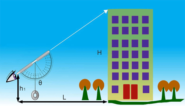
The height is calculated as:
- \(h_1\) = height of clinometer
- \(L\) = horizontal distance
- \(\theta\) = measured angle
Sensitivity coefficients:
- For \(h_1\): \(\frac{\partial H}{\partial h_1} = 1\)
- For \(L\): \(\frac{\partial H}{\partial L} = \tan(\theta)\)
- For \(\theta\): \(\frac{\partial H}{\partial \theta} = L \cdot \sec^2(\theta)\)
Interpretation:
A small error in \(\theta\) can cause a large error in \(H\), especially at steep angles.
Visualizing Sensitivity
The blog post shows how the sensitivity coefficient for angle (\(\theta\)) increases rapidly as the angle increases. This means that at higher angles, even a small error in measuring \(\theta\) can lead to a large error in the calculated height.

Special Case: Temperature Effects
For measurements affected by temperature, such as thermal expansion:
- \(\alpha\) = coefficient of thermal expansion
- \(L\) = measured length
A small temperature change can have a significant effect on long measurements.
Practical Tips
- Always check units: Sensitivity coefficients may have units. Make sure all uncertainties are in compatible units before combining.
- Nonlinear equations: For nonlinear relationships, sensitivity coefficients can change depending on the value of the input. Evaluate them at the expected value or at the uncertainty limit for worst-case analysis.
- Environmental factors: Consider temperature, humidity, and other environmental effects in your uncertainty budget.
Uncertainty Budget Example
| Source | Value | Distribution | Divisor | Sensitivity | Standard Uncertainty |
|---|---|---|---|---|---|
| \(L\) | \(\pm 50.5\) mm | Normal (95%) | 2 | 1.6 | 40.4 mm |
| \(h_1\) | \(\pm 8.75\) mm | Normal (95%) | 2 | 1.0 | 4.4 mm |
| \(\theta\) | \(\pm 1^\circ\) | Normal | 1 | 632 mm/deg | 632 mm |
Combined standard uncertainty:
Summary
- Sensitivity coefficients show how much each input affects the output.
- Use partial derivatives to calculate sensitivity coefficients for each input.
- Always include sensitivity coefficients in your uncertainty budget.
- Pay special attention to inputs with large sensitivity coefficients—they dominate the uncertainty.
Formula reference
For each source, \(u_i = (\text{Value } a_i / \text{Divisor}) \times c_i\); combined \(u_c(y) = \sqrt{\sum u_i^2}\) (RSS, uncorrelated inputs); expanded \(U = k \cdot u_c(y)\) with \(k=2\) for ~95% confidence. Divisors: normal (\(k=2\)) → 2, rectangular → \(\sqrt{3}\), triangular → \(\sqrt{6}\), already-standard (\(k=1\)) → 1. Worked budget tables using this exact recipe live in Uncertainty 101 and the checklist.