Simple example of mechanical measurement with uncertainty analysis#
Source:#
1. Decide what you measure and what you need to find out from measurements#
In this example we want to measure length of a string and we decide to use tape measure. we want to know the length and we want to estimate how good we measure it.
First step: think. what are the possible errors?
errors due to the measurement device:
does the tape need calibration? is it calibrated already? what is the uncertainty of the calibration (it’s an imported uncertainty). how much could calibration change since it was performed last time?
is the tape needs stretching? alignment? attachment?
could it bend? is bending causing shortening?
what is the resolution? what is the smallest change we can notice using this tape? how small are divisions on the tape?
measurement errors due to the item being measured:
can this string be streteched and straight?
can it be under-stretched? curly?
does the temperature/humidity of the environment affect measured length?
can we easily define the ends of the string? can we attack it to the tape measure?
errors due to the measurement process and the person making measurements:
how well can you line up the beginning and the end of the string? do you see it well? can you align it?
how repeatable is your reading of the point between divisions?
can you think of additional error sources?
2. Measure#
measure and record your results clearly. state the date, the time, the serial number of the tape measure you use, an id of the string you measure. write down how the measurements are performed, how participated, environmental conditions (temperature, humidity, etc.), all other relevant remarks if you use code, Excel, etc.
to be extra careful, repeat your measurement several times, attach the string every time.
record all the measurements and take an average and standard deviation. e.g. 5.017 m and 0.0021 m, respectively
3. Estimate uncertainty, source by source, standartize each#
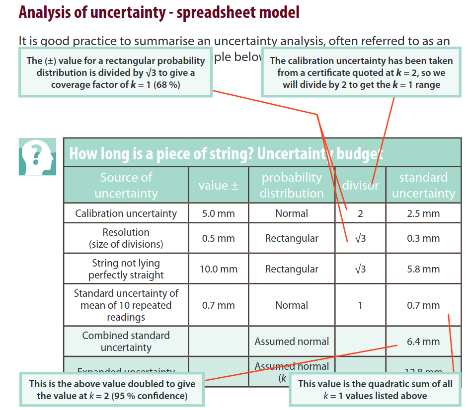
calibration: the tape measure has to be calibrated. let’s assume we got a calibrated one and it says: 0.1% of reading, in calibration a normal distribution was used (it’s written usually, \(k\) - cover factor is 2, i.e. normal distribution). So we can take our measurement best estimate, the average, \(5.017 \times 0.0001 / 2 \approx 2.5\) mm, \(u_{\mathrm{cal}} = 2.5 \) mm.
divisions of the tape are millimeters, i.e. resolution is 1 mm, reading to the nearest one leaves the
resolution errorwhich is \(\pm 0.5\) mm. let’s assume that all values whithin this range are equally probable, i.e. we assume rectangular or uniform distribution, to find standard uncertainy from the resolution error we divide by the cover coefficient of uniform distribution, \(\sqrt{3}\), \(u_{\mathrm{res}} = 0.5 / \sqrt{3} \approx 0.3\) mmalthough we can stretch the string, and the tape, probably it would have some bends along the way, so we could assume that we underestimate the actual, true length. let’s assume we give it 0.2% of the measurement. so we get 10 mm. we can assume it is also uniformly distributed, so we take \(u = 10/\sqrt{3} = 5.8\) mm (rounded to the nearest 0.1 mm)
All these above are Type B sources, the following is Type A:
we need to get standard uncertainty of our repeated measurements with average and standard derviation. we calculate the standard uncertainty of the mean of the 10 readings: $\( s/\sqrt{n} = 2.1/\sqrt{10} = 0.7 \)mm (to one decimal place)
4. Decide whether the different error sources are independent of each other#
let’s assume and write down these are independent
5. Calculate the result of your measurement#
In this simple case it is to write down the average and take into account the corrections you assumed: e.g. that the tape and string are straight and parallel.
6. Find the combined uncertainty from all the sources#
7. Express your result using the standard uncertainty and cover factor, write the confidence level for the cover factor#
For a coverage of \(k=2\), we multiply the \(u\) by 2 and get \(u = 2 \times 6.4 = 12.8\) mm with the confidence level of 95% (coverage factor, see the lecture about Gaussian distribution)