Using FFT the right way to find the correct spectrum

from numpy import *
from numpy.fft import fft
import matplotlib.pyplot as plt
%matplotlib inline

# redefine default figure size and fonts
import matplotlib as mpl
mpl.rc('font', size=16)
mpl.rc('figure',figsize=(12,10))
mpl.rc('lines', linewidth=1, color='lightblue',linestyle=':',marker='o')

import sys
sys.path.append('../scripts')
from signal_processing import create_signal, spectrum

fs = 30 # sampling frequency, Hz
N = 256 # number of sampling points

t,y = create_signal(fs,N)

def plot_signal_with_fft(t,y,fs,N):
    """ plots a signal in time domain and its spectrum using 
    sampling frequency fs and number of points N
    """

    T = N/fs # sampling period
    y -= y.mean() # remove DC
    frq,Y = spectrum(y,fs) # FFT(sampled signal)
    
    # Plot
    fig, ax = plt.subplots(2,1)
    ax[0].plot(t,y,'b.')
    ax[0].plot(t,y,':',color='lightgray')
    ax[0].set_xlabel('$t$ [s]')
    ax[0].set_ylabel('Y [V]')
    ax[0].plot(t[0],y[0],'ro')
    ax[0].plot(t[-1],y[-1],'ro')
    ax[0].grid()

    
    ax[1].plot(frq,abs(Y),'r') # plotting the spectrum
    ax[1].set_xlabel('$f$ (Hz)')
    ax[1].set_ylabel('$|Y(f)|$')
    lgnd = str(r'N = %d, f = %d Hz' % (N,fs))
    ax[1].legend([lgnd],loc='best')
    ax[1].grid()

### Note we remove DC right before the spectrum

plot_signal_with_fft(t,y,fs,N)

---------------------------------------------------------------------------
AttributeError                            Traceback (most recent call last)
Cell In[6], line 1
----> 1 plot_signal_with_fft(t,y,fs,N)

Cell In[4], line 8, in plot_signal_with_fft(t, y, fs, N)
      6 T = N/fs # sampling period
      7 y -= y.mean() # remove DC
----> 8 frq,Y = spectrum(y,fs) # FFT(sampled signal)
     10 # Plot
     11 fig, ax = plt.subplots(2,1)

File ~/Documents/repos/engineering_experiments_measurements_course/book/signal_processing/../scripts/signal_processing.py:36, in spectrum(y, Fs)
     34 T = n/Fs
     35 frq = k/T  # two sides frequency range
---> 36 frq = frq[range(np.int(n/2))]  # one side frequency range
     37 Y = 2*fft.fft(y)/n  # fft computing and normalization
     38 Y = Y[range(np.int(n/2))]

File ~/mambaforge/envs/mdd/lib/python3.10/site-packages/numpy/__init__.py:324, in __getattr__(attr)
    319     warnings.warn(
    320         f"In the future `np.{attr}` will be defined as the "
    321         "corresponding NumPy scalar.", FutureWarning, stacklevel=2)
    323 if attr in __former_attrs__:
--> 324     raise AttributeError(__former_attrs__[attr])
    326 if attr == 'testing':
    327     import numpy.testing as testing

AttributeError: module 'numpy' has no attribute 'int'.
`np.int` was a deprecated alias for the builtin `int`. To avoid this error in existing code, use `int` by itself. Doing this will not modify any behavior and is safe. When replacing `np.int`, you may wish to use e.g. `np.int64` or `np.int32` to specify the precision. If you wish to review your current use, check the release note link for additional information.
The aliases was originally deprecated in NumPy 1.20; for more details and guidance see the original release note at:
    https://numpy.org/devdocs/release/1.20.0-notes.html#deprecations

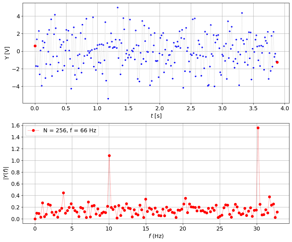
fs = 66 # sampling frequency, Hz
N = 256 # number of sampling points

t,y = create_signal(fs,N)
plot_signal_with_fft(t,y,fs,N)

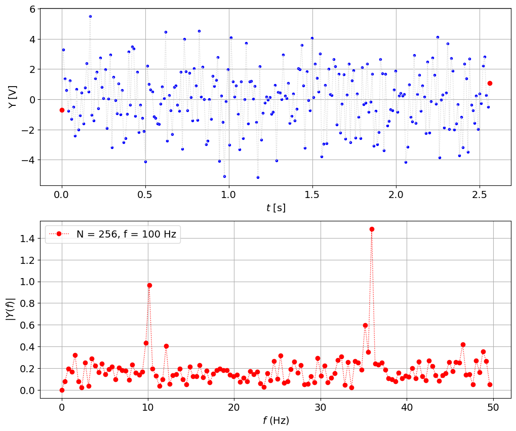
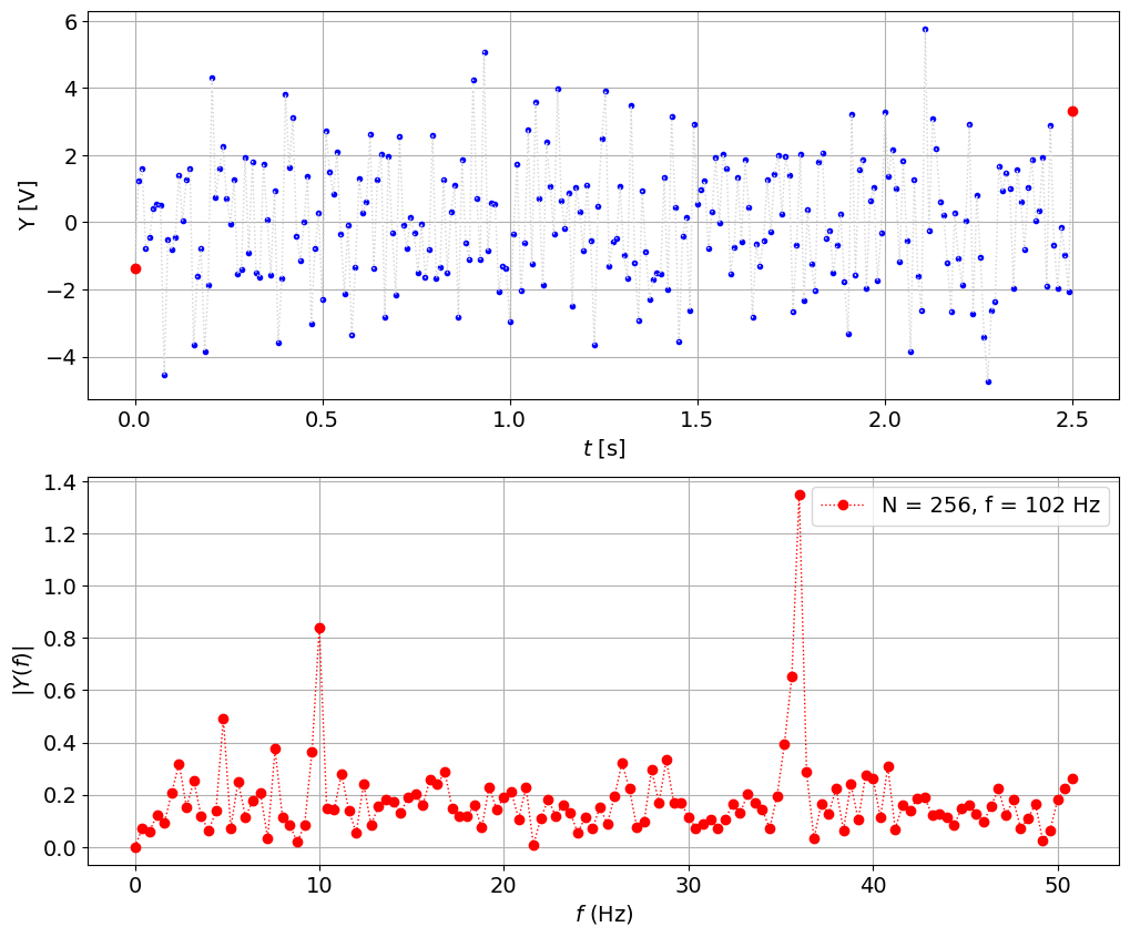
fs = 100 # sampling frequency, Hz
N = 256 # number of sampling points

t,y = create_signal(fs,N)
plot_signal_with_fft(t,y,fs,N)

fs = 500 # sampling frequency, Hz
N = 256 # number of sampling points

t,y = create_signal(fs,N)
plot_signal_with_fft(t,y,fs,N)

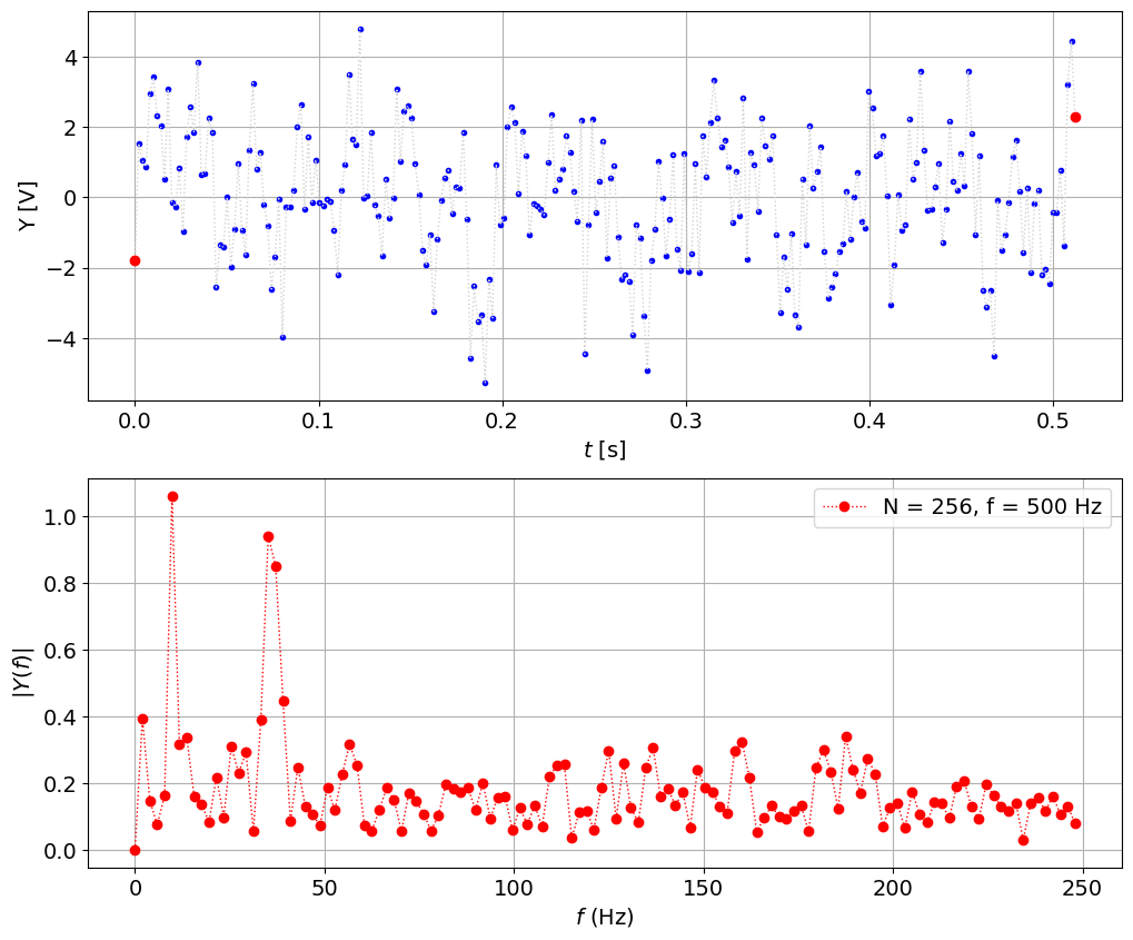
• Very poor frequency resolution, \(\Delta f = 1/T = fs/N = 500 / 256 = 1.95 Hz\) versus \(\Delta f = 100 / 256 = 0.39 Hz\)

• peaks are at 9.76 Hz and 35.2 Hz

• wasting a lot of frequency axis above 2 * 35.7

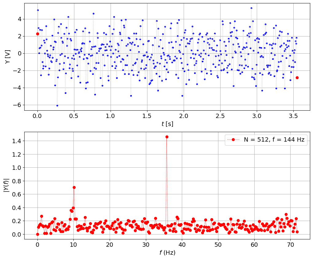
So the problem is still there:

the peak is now shifted to 35.5 Hz, let’s see: when we sampled at 30 we got aliased 35.5 - 30 = 5.5 Hz. Seems correct, when we sampled at 66 it was above 2/3f but below 2f, so 66 - 35.5 = 30.5 Hz, also seem to fit. So now we have explained (!) the previous results and we believe that hte signal has 10 Hz and 35.5 Hz (approximately) and 100 Hz is good enough but we could improve it by going slightly above Nyquist 2*35.5 = 71 Hz, and also try to fix the number of points such that we get integer number of periods. It’s imposible since we have two frequencies, but at least we can try to get it close enough: 1/10 = 0.1 sec so we could do 256 * 0.1 = 25.6 Hz or X times that = 25.6 * 3 = 102.4 - could be too close let’s try:

fs = 102.4 # sampling frequency, Hz
N = 256 # number of sampling points
t,y = create_signal(fs,N)
plot_signal_with_fft(t,y,fs,N)

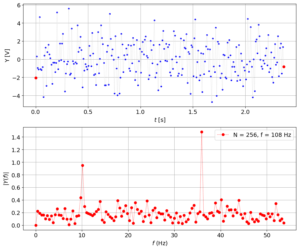
Then the same principle to get better 35.5 Hz 1/35.5 * 256 = 7.21 * 15 = 108.16 Hz

fs = 108.16 # sampling frequency, Hz
N = 256 # number of sampling points
t,y = create_signal(fs,N)
plot_signal_with_fft(t,y,fs,N)

fs = 144.22 # sampling frequency, Hz
N = 512 # number of sampling points
t,y = create_signal(fs,N)
plot_signal_with_fft(t,y,fs,N)

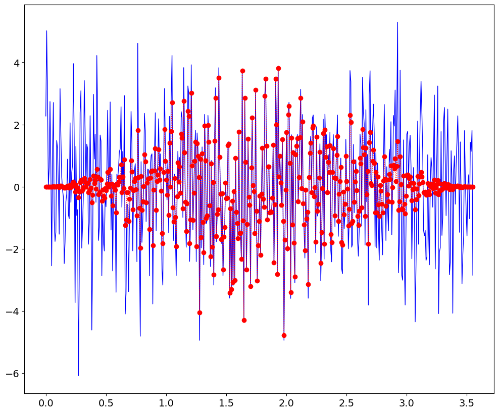
Use windowing or low-pass filtering

from scipy.signal import hann  # Hanning window

# we made a mistake with the DC

DC = y.mean()
y -= DC


yh = y*hann(len(y))

plt.plot(t,y,'b-',t,yh,'r') 

[<matplotlib.lines.Line2D at 0x7f0a0ba321c0>,
 <matplotlib.lines.Line2D at 0x7f0a0ba32400>]

frq,Y = spectrum(yh,fs)

Y = abs(Y)*sqrt(8./3.)# /(N/2) 

plt.plot(frq,Y)

[<matplotlib.lines.Line2D at 0x7f0a0bb3f280>]

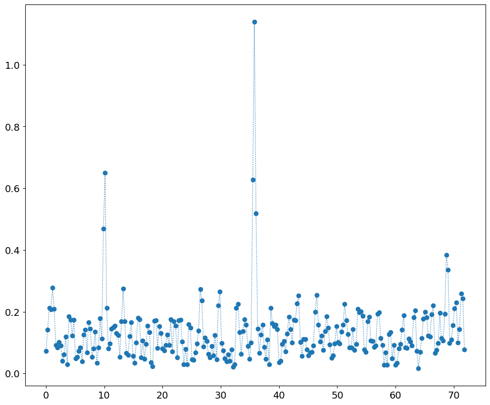
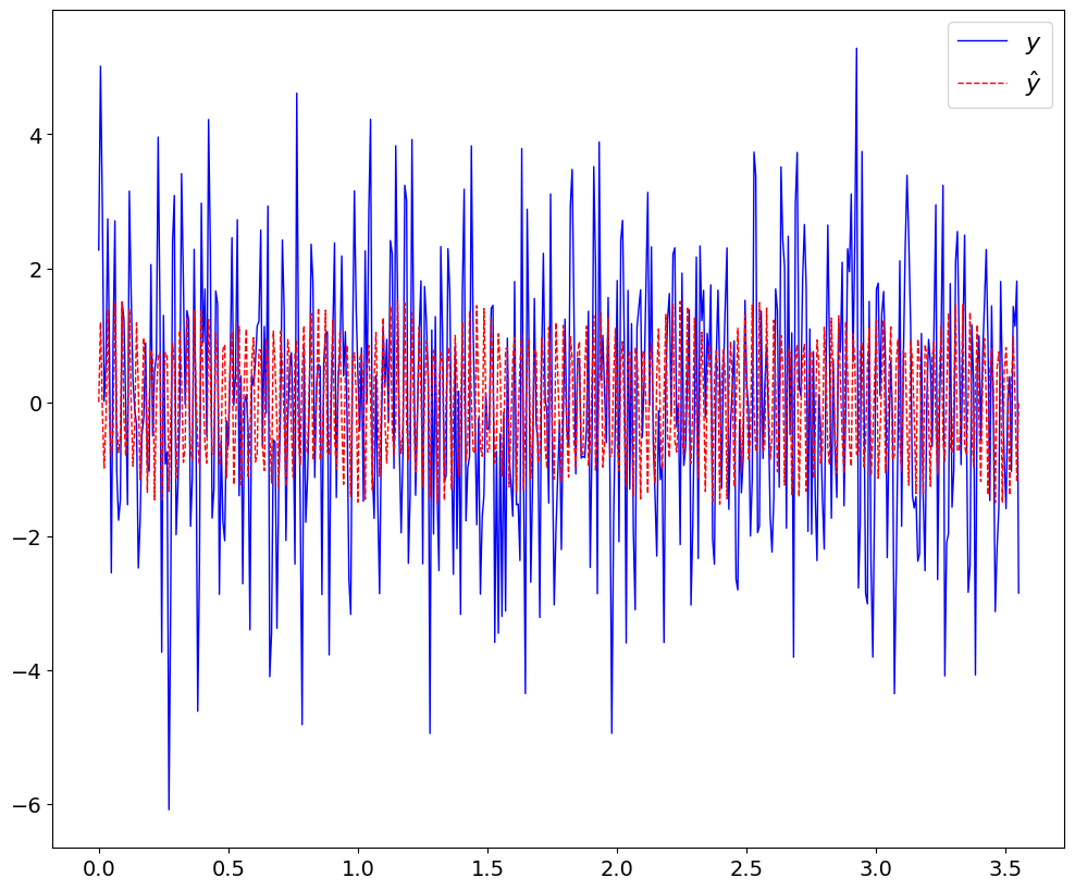
let’s try to reconstruct

a1,f1 = Y.max(),frq[Y.argmax()]
print (a1,f1)
b = Y.copy()
b[:Y.argmax()+10] = 0 # remove the first peak
a2,f2 = b.max(),frq[b.argmax()]
print (a2,f2)

1.1387020742945604 35.7733203125
0.3830241283109943 68.72984375

yhat = DC + a1*sin(2*pi*f1*t) + a2*sin(2*pi*f2*t)
plt.plot(t,y+DC,'b-',t,yhat,'r--');
plt.legend(('$y$','$\hat{y}$'),fontsize=16);