1st order dynamic system

Following the example of Prof. Cimbala ME 345 course

import numpy as np
import matplotlib.pyplot as plt
import matplotlib as mpl
mpl.rcParams['lines.linewidth']=2
mpl.rcParams['lines.color']='r'
mpl.rcParams['figure.figsize']=(10,12)
mpl.rcParams['font.size']=14
mpl.rcParams['axes.labelsize']=16

T = 1.
t = np.arange(0,10*T,.0001)
t_T = t/T

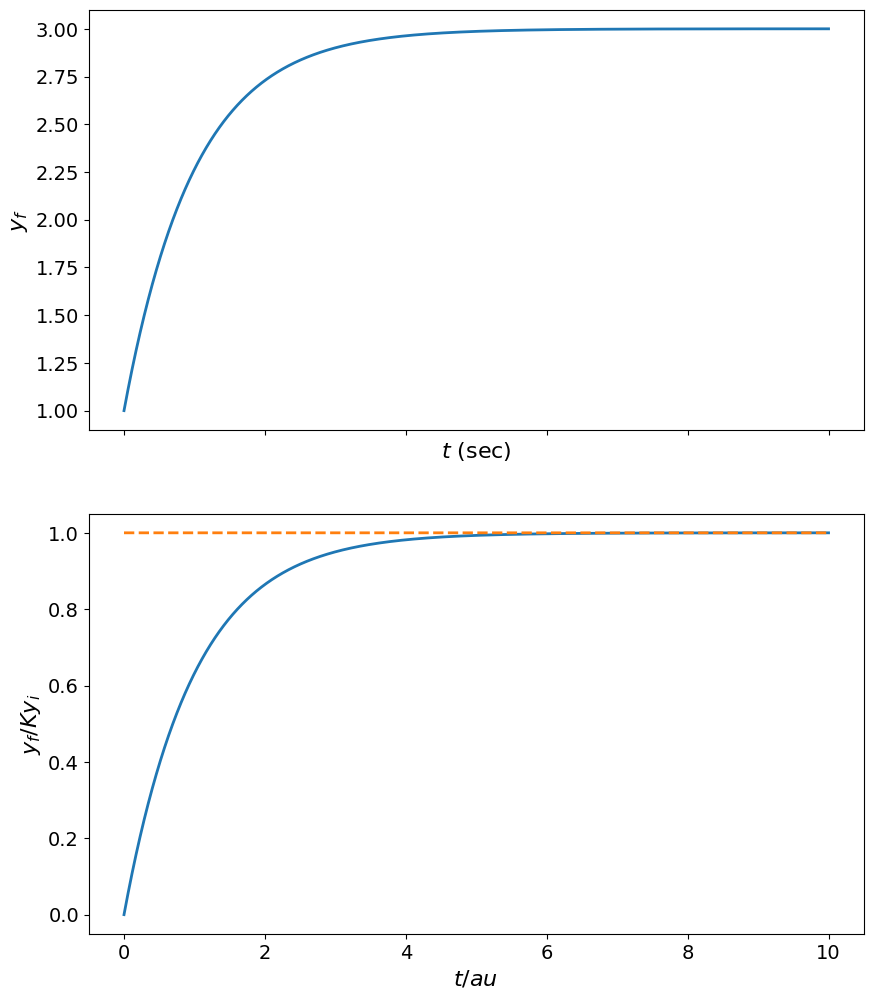
# Step function

# for a step function, take user input on final and initial values.
y_i = 1.0
y_f = 3.0

y_step_norm =  (1 - np.exp(-t_T))
y_step = (y_f-y_i)*y_step_norm + y_i

fig,ax = plt.subplots(nrows=2,sharex=True)
ax[0].plot(t, y_step)
ax[0].set_xlabel('$t$ (sec)')
ax[0].set_ylabel('$y_f$')

ax[1].plot(t_T,y_step_norm)
ax[1].plot(t_T,np.ones(t_T.shape),'--')
ax[1].set_xlabel('$t/\tau$ ');
ax[1].set_ylabel('$y_f/Ky_i$');

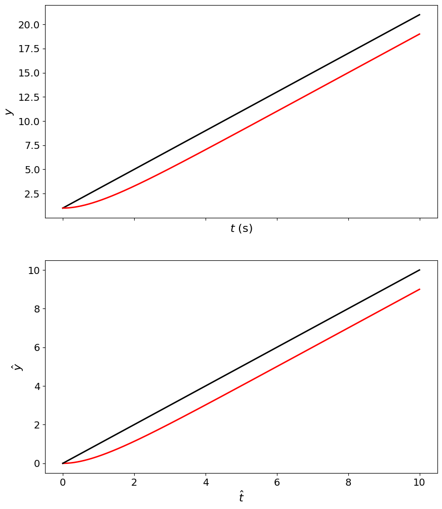
y_i_ramp = 1.
A = 2.

# determine actual ramp function. 
y_ideal_ramp = A*t + y_i_ramp;
y_ramp_norm = (t - T*(1-np.exp(-t_T)));
y_ramp = A*y_ramp_norm + y_i_ramp;

fig,ax = plt.subplots(nrows=2,sharex=True)
# figure(figsize=(10,8))
ax[0].plot(t, y_ideal_ramp, 'k', t, y_ramp, 'r')
ax[0].set_xlabel('$t$ (s)')
ax[0].set_ylabel('$y$')

ax[1].plot(t_T, y_ramp_norm,'r', t_T, t, 'k')
ax[1].set_xlabel('$\hat{t}$ ')
ax[1].set_ylabel('$\hat{y}$')

Text(0, 0.5, '$\\hat{y}$')

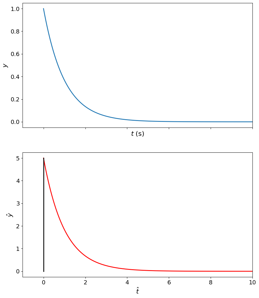
y_i_impulse = 0.;
y_f_impulse = 5.;

y_impulse_norm = (1./T)*np.exp(-t_T);
y_impulse = y_impulse_norm * (y_f_impulse-y_i_impulse) + y_i_impulse;

fig,ax = plt.subplots(nrows=2,sharex=True)
# figure(figsize=(10,8))
ax[0].plot(t_T, y_impulse_norm)
ax[0].set_xlabel('$t$ (s)');
ax[0].set_ylabel('$y$');

ax[1].plot(t,y_impulse,'r',[0.,0.],[y_i_impulse,y_f_impulse],'k')
ax[1].set_xlim([-T,10*T])
ax[1].set_xlabel('$\hat{t}$ ');
ax[1].set_ylabel('$\hat{y}$');