Example of pre-measurement design

Pressure transducer choice of parameters

We require to choose a pressure transduced such that we could measure a signal up to 100 Hz with a dynamic error of up to 5%.

The pressure transducers available in the lab is measured to have damping of \(\zeta = 0.5\) and ringing frequency of 1200 Hz.

%pylab inline
from scipy import signal
import numpy as np

%pylab is deprecated, use %matplotlib inline and import the required libraries.
Populating the interactive namespace from numpy and matplotlib

# Define transfer function
fd = 1200 # Hz
fn = fd/(np.sqrt(1-0.5**2))
wn = fn/(2*np.pi) # rad/s
z=0.5     # damping
k = 1 		# sensitivity


sys = signal.lti(k*wn**2,[1,2*z*wn, wn**2])

# step function output
t,y = sys.step(N=1000)

figure(figsize=(8,6))
plot(t,y)
title('Step response of a pressure transducer')
xlabel('$t$ [sec]')
ylabel('E [V]')

Text(0, 0.5, 'E [V]')

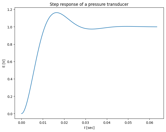
# note that sampling is sufficient, if not we need to apply the D/A reconstruction
# or interpolations, which will add more noise and uncertainty to the system identification

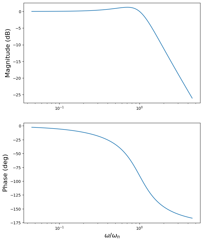
# Create Bode plot
w, mag, phase = signal.bode(sys)

fig,ax = subplots(2,1,figsize=(8,10))
ax[0].semilogx(w/wn, mag)    # Bode magnitude plot
# ax[0].plot(w/wn,mag)
ax[0].set_ylabel('Magnitude (dB)',fontsize=16)
ax[1].semilogx(w/wn, phase)  # Bode phase plot
# ax[1].plot(w/wn, phase)  # Bode phase plot
ax[1].set_ylabel('Phase (deg)',fontsize=16)
ax[1].set_xlabel('$\omega/\omega_n$',fontsize=16)
# fig.savefig('bode_pressure_transducer.png',dpi=200)

Text(0.5, 0, '$\\omega/\\omega_n$')