Step responses of dynamical systems

#!/usr/bin/env python
from numpy import *
from matplotlib import pyplot as plt
from scipy import signal
%matplotlib inline

import matplotlib as mpl
mpl.rcParams['lines.linewidth']=2
mpl.rcParams['lines.color']='r'
mpl.rcParams['figure.figsize']=(10,10)
mpl.rcParams['font.size']=14
mpl.rcParams['axes.labelsize']=20
 
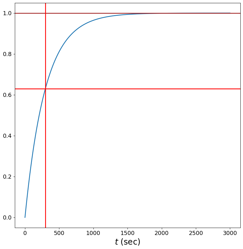
tau = 5.0*60   # 5 minutes
h_times = arange(0.0, 10*tau, 0.1)
 
sys = signal.lti(1,[1,1.0/tau])
 
step_response = sys.step(T=h_times)[1]
plt.plot(h_times, step_response/step_response[-1])    # normalized
plt.axhline(1.0, color='brown')
plt.axhline(0.63, color='red')
plt.axvline(tau, color='red')
plt.xlabel(r'$t$ (sec)')
# plt.title('Step response')
# plt.show()

Text(0.5, 0, '$t$ (sec)')

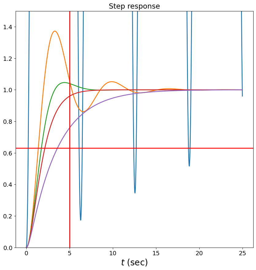
tau = 5.0   # 5 sec
h_times = arange(0.0, 5*tau, 0.01)

omega_n = 1 # rad/s

for zeta in [0.001,0.3,0.7,1,1.8]:
    # zeta = 0.1  # damping
    sys = signal.lti(1,[1, 2*zeta/omega_n, 1./omega_n**2])
    step_response = sys.step(T=h_times)[1]
    plt.plot(h_times, step_response/step_response[-2])    # normalized
    
plt.axhline(0.63, color='red')
plt.axvline(tau, color='red')    
plt.xlabel(r'$t$ (sec)')
plt.title('Step response')
plt.ylim([0,1.5])
plt.show()