Tutorial: Your First Tracking (GUI, 10 minutes)¶

Track real particles in 3D using the example bundled with openptv2. No data to download, no parameters to change.

You will: open the test_cavity example, detect particles, match them across 4 cameras, track them over time, and see the trajectories.

Watch the whole walkthrough first (30 seconds, recorded from the real GUI):

GUI walkthrough animation

Before you start¶

openptv2 installed with the GUI:
```
pip install "openptv2[gui]"
```
A checkout of the openptv2 repository (the example lives in test_data/test_cavity). If you installed from PyPI without the source, clone it:
```
git clone https://github.com/alexlib/openptv2.git
cd openptv2
```

Step 1: Open the example¶

openptv2-gui -w test_data/test_cavity/parameters_Run1.yaml

The GUI opens showing 4 camera views of a lid-driven cavity experiment (frames 10000–10004).

What it does: -w points the GUI at one experiment. Passing a YAML file makes that run active; passing a directory opens the first run found there. Everything the GUI needs — image paths, calibrations, detection and tracking settings — lives in that single YAML file.

Parameters in YAML: the whole parameters_Run1.yaml. Each Run in the left-hand tree is one parameters_*.yaml file in the folder (Run1 → parameters_Run1.yaml). Right-click a run for Main / Calibration / Tracking parameters dialogs; edits are saved back to its YAML.

GUI with example open

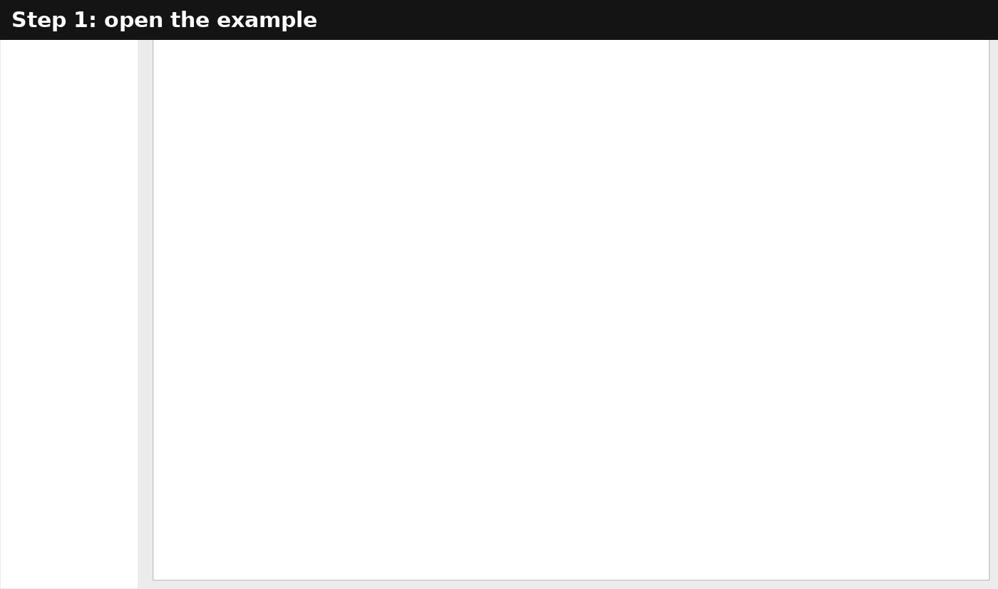
Step 2: Load parameters — Start → Init / Reload¶

Click Start → Init / Reload in the menu bar.

Success looks like this in the console:

Read all the parameters and calibrations successfully

The 4 camera views now show the first frame. If you see this message, everything else in this tutorial will work.

What it does: reads the active YAML, loads the 4 camera calibrations (cal/camN.tif.ori + .addpar) and the current frame's images (ptv.img_name). No options — it either loads cleanly or reports what is missing.

Parameters in YAML: ptv section (img_name, imx/imy, multimedia mmp_n1/n2/n3, mmp_d) and cal_ori section (calibration file locations).

GUI after Init / Reload

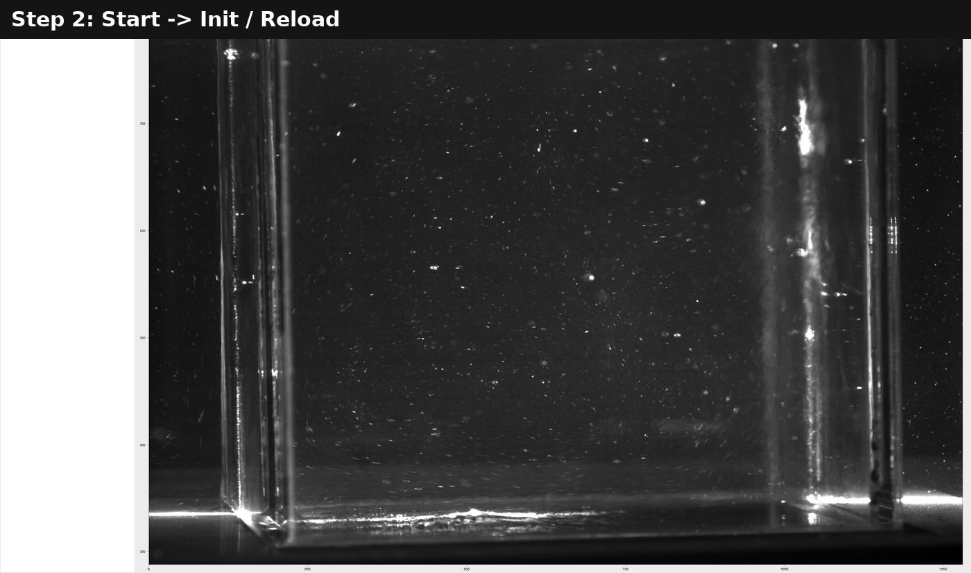
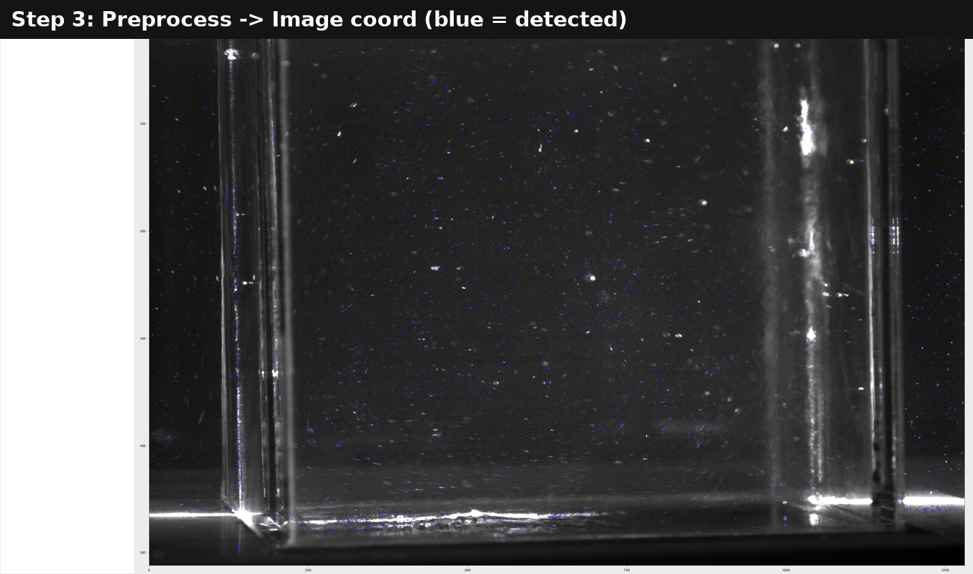
Step 3: Detect particles — Preprocess → Image coord¶

Click Preprocess → Image coord.

The console prints:

Start detection
Detection finished

Each camera view fills with blue crosses — one per detected particle (several hundred per camera). This is 2D detection: finding bright spots in each image.

What it does: thresholds each image and keeps blobs that look like particles (bright enough, right size). Too few crosses → lower the threshold; merges and streaks → raise it or tighten the size bounds.

Parameters in YAML (targ_rec section): gvthres (brightness threshold, one per camera), sumg_min (minimum total brightness), nnmin/nnmax (pixel count), nxmin/nxmax and nymin/nymax (width/height bounds). Edit via right-click Run1 → Main parameters.

GUI after Image coord: blue detection crosses

Step 4: Match across cameras — Preprocess → Correspondences¶

Click Preprocess → Correspondences.

The console prints:

correspondence proc started

New crosses appear in yellow (seen in 2 cameras), green (3 cameras), and red (all 4 cameras). This is stereo matching: the same physical particle found in multiple views is triangulated into a 3D position.

What it does: for each detection, searches the other cameras along its epipolar line; consistent sightings become one 3D point. Detections and 3D points are written to the run's zarr store (run.zarr). Mostly blue with little color → calibration or tolerances need work, not the detection threshold.

Parameters in YAML (criteria section): eps0 (epipolar tolerance), corrmin (minimum match quality), cn/cnx/cny/csumg (center tolerances), X_lay/Zmin_lay/Zmax_lay (allowed 3D volume). The ptv section's mmp_* values describe the air–glass–water optics and must match your tank.

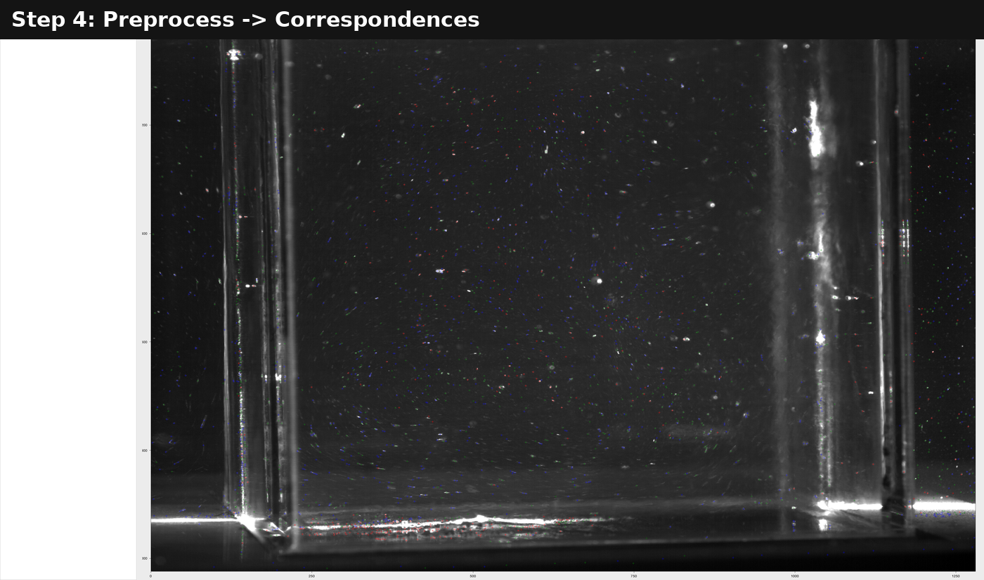
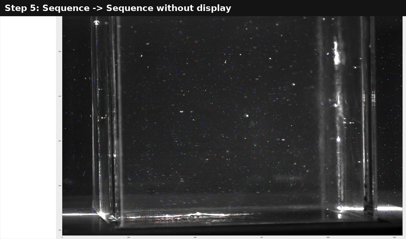
GUI after Correspondences: matched particles in color

Step 5: Process all frames — Sequence → Sequence without display¶

Click Sequence → Sequence without display.

This repeats Steps 3–4 for every frame (10000–10004). It takes under a minute. Per-frame detections and 3D points accumulate in the run's zarr store (run.zarr).

What it does: runs the active sequence plugin over the whole frame range — same detection + correspondence code as Steps 3–4, no new science, just all frames.

Parameters in YAML (sequence section): base_name (image filename pattern per camera), first/last (frame range). To process more frames, extend last here — or pass --first/--last to pyptv_batch.

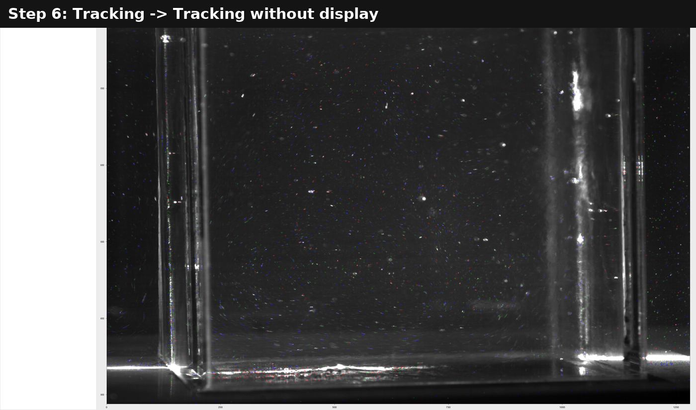
GUI after Sequence: all frames processed

Step 6: Track over time — Tracking → Tracking without display¶

Click Tracking → Tracking without display.

The console prints:

tracking without display finished

Particles are now linked frame-to-frame into trajectories, stored as linkage in the run's zarr store (run.zarr, sealed into trajectories automatically). Expect a few hundred trajectories over these frames.

What it does: predicts where each 3D particle should appear next frame and links nearest matches into paths. Short/broken tracks → widen the velocity box or raise dacc; wrong connections → narrow them.

Parameters in YAML (track section): dvxmin/dvxmax, dvymin/dvymax, dvzmin/dvzmax (velocity search box per axis), dacc (acceleration tolerance), angle (max direction change), flagNewParticles (start tracks on unmatched particles). The tracker itself is chosen in plugins.selected_tracking (this example: default). Edit via right-click Run1 → Tracking parameters. The warmup tutorial derives these from your data automatically.

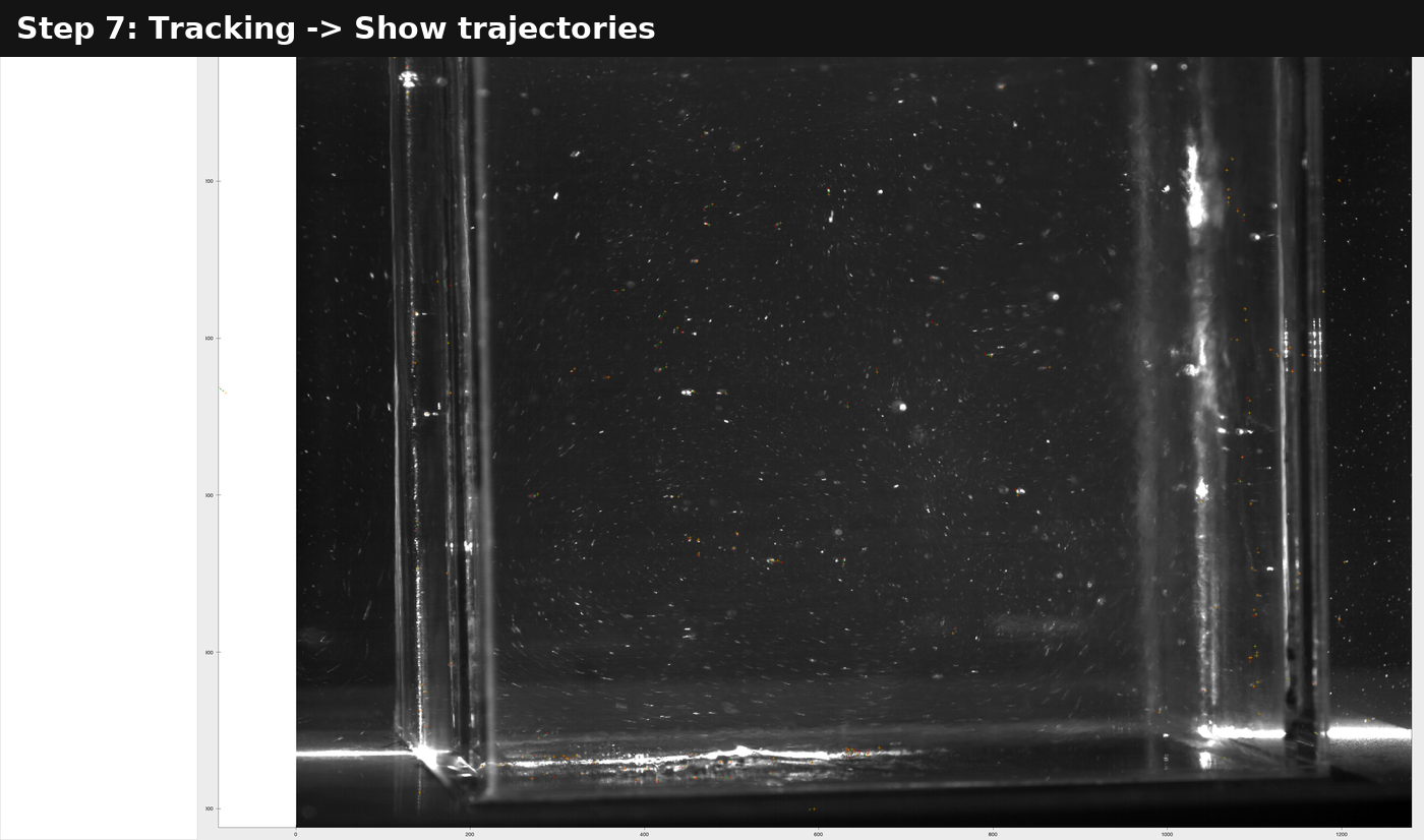
GUI after Tracking: linked trajectories

Step 7: See the trajectories — Tracking → Show trajectories¶

Click Tracking → Show trajectories to plot the 3D paths.

What it does: reads the sealed trajectories from the zarr store and draws them on the camera views — red heads, green tails, orange ends. Pure visualization: no parameters, nothing is recomputed.

GUI trajectories: heads (red), tails (green), ends (orange)

You just ran a full 3D-PTV pipeline: detect → match → track → visualize.

If something goes wrong¶

Symptom	Fix
GUI fails with `No module named 'traitsui'`	You installed without the GUI extra. Run `pip install "openptv2[gui]"`.
`Init / Reload` reports a missing image	Check you launched from the repository root so relative paths in the YAML resolve.
No crosses after Image coord	The example threshold is pre-tuned; make sure Step 2 succeeded first.

Same run without the GUI¶

Every click above has a command-line equivalent (useful on servers). From the repository root:

# Steps 3–5 (detection + correspondences, all frames)
pyptv_batch --workdir=test_data/test_cavity --first=10000 --last=10001 --mode=sequence

# Step 6 (tracking)
pyptv_batch --workdir=test_data/test_cavity --first=10000 --last=10001 --mode=tracking

Regenerating these screenshots¶

All images and the animation on this page are recorded from the real GUI by docs/tutorials/record_gui_tutorial.py, which drives the same menu handlers and captures the window after each step. Re-run it from the repository root after GUI changes:

uv run python docs/tutorials/record_gui_tutorial.py

Where to go next¶

Tracking Pipeline & Results — what each step does and where result files land.
Command-Line Batch Processing — headless runs on your own data.
Plate Calibration How-To — calibrating your own cameras (only needed for new experiments, not this example).
Lid-Driven Cavity Flow — the advanced, scripted version of this example (autocalibration, self-calibration, warmup).