Outliers#
import numpy as np
import matplotlib.pyplot as pl
%matplotlib inline

import matplotlib as mpl
mpl.rcParams['lines.linewidth']=2
mpl.rcParams['lines.color']='r'
mpl.rcParams['figure.figsize']=(10,8)
mpl.rcParams['font.size']=14
mpl.rcParams['axes.labelsize']=20
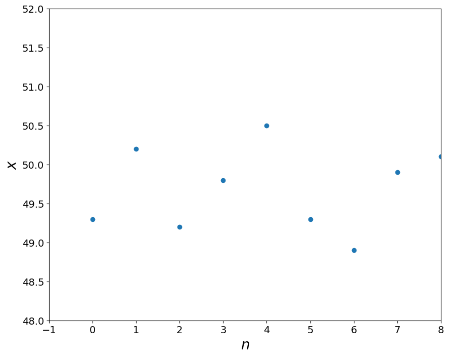
Single variable, \(x\)#
x = np.array([49.3,50.2,49.2,49.8,50.5,49.3,48.9,49.9,50.1,49.2])
pl.figure()
pl.plot(x,'o')
pl.xlim([-1,8])
pl.ylim([48,52])
pl.ylabel('$x$')
pl.xlabel('$n$')
Text(0.5, 0, '$n$')
We use modified Thompson test (based on Student’s t-distribution)#
Sort the values#
x.sort()
x
array([48.9, 49.2, 49.2, 49.3, 49.3, 49.8, 49.9, 50.1, 50.2, 50.5])
pl.plot(x,'o')
pl.xlim([-1,8])
pl.ylim([48,52])
pl.ylabel('$x$')
pl.xlabel('$n$')
Text(0.5, 0, '$n$')
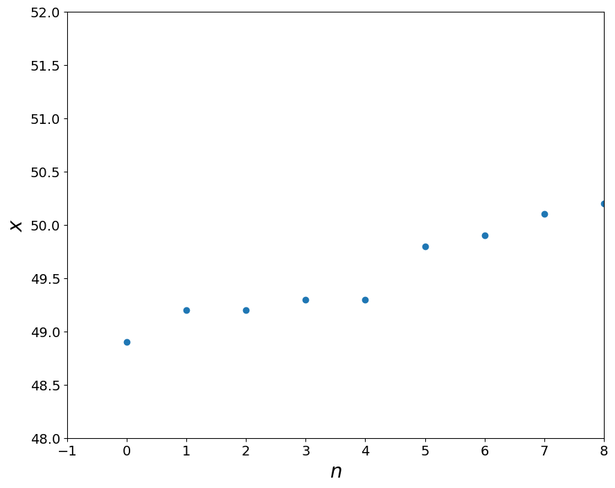
Note: we suspect in the sorted list of values the first and the last
get the sample mean and sample standard deviation, get deviations#
x_mean = np.mean(x)
x_std = np.std(x,ddof=1)
print( x_mean)
print (x_std)
49.64
0.5295700562196137
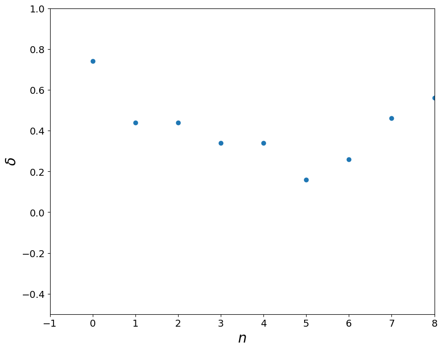
\(\delta_i = | x - x_i |\)
delta = abs(x - x_mean)
pl.plot(delta,'o')
pl.xlim([-1,8])
pl.ylim([-.5,1])
pl.ylabel('$\delta$')
pl.xlabel('$n$')
print (delta[0],delta[-1])
0.740000000000002 0.8599999999999994
<>:5: SyntaxWarning: invalid escape sequence '\d'
<>:5: SyntaxWarning: invalid escape sequence '\d'
/tmp/ipykernel_276332/2879644948.py:5: SyntaxWarning: invalid escape sequence '\d'
  pl.ylabel('$\delta$')