Fourier transforms with windowing

import matplotlib.pyplot as plt
import numpy as np
%matplotlib inline

from numpy import fft

import matplotlib as mpl
mpl.rc('font', size=14)
mpl.rc('figure',figsize=(12,10))

# Given:

f_s = 100.0 # sampling frequency (Hz)
T = 3.0 # total actual sample time (s)

g = np.loadtxt('../data/FFT_Example_data_with_window.txt')
# add noise
for i in range(10):
    g += np.random.rand(g.shape[0])

# Calculate
N = f_s*T  #total actual number of data points
del_t = 1./f_s  #(s)
del_f = 1./T  #(Hz)
f_fold = f_s/2.  #folding frequency = max frequency of FFT (Hz)
N_freq = N/2.  #number of discrete frequencies

t = np.arange(0.0,T+del_t,del_t)  #time, t (s)

g += 1.2*np.sin(2*np.pi*10*t)

frequency = np.arange(0,f_fold,del_f)  #frequency (Hz)
G = fft.fft(g) # FFT 
Magnitude = np.abs(G)/(N/2.)  #|F|/(N/2)
Magnitude[0] = Magnitude[0]/2
len_loc, = Magnitude.shape
A = Magnitude[0:np.int(round(len_loc/2))]
Freq = frequency[0:np.int(round(len_loc/2))]

---------------------------------------------------------------------------
AttributeError                            Traceback (most recent call last)
Cell In[4], line 6
      4 Magnitude[0] = Magnitude[0]/2
      5 len_loc, = Magnitude.shape
----> 6 A = Magnitude[0:np.int(round(len_loc/2))]
      7 Freq = frequency[0:np.int(round(len_loc/2))]

File ~/miniforge3/envs/book/lib/python3.11/site-packages/numpy/__init__.py:778, in __getattr__(attr)
    773     warnings.warn(
    774         f"In the future `np.{attr}` will be defined as the "
    775         "corresponding NumPy scalar.", FutureWarning, stacklevel=2)
    777 if attr in __former_attrs__:
--> 778     raise AttributeError(__former_attrs__[attr], name=None)
    780 if attr in __expired_attributes__:
    781     raise AttributeError(
    782         f"`np.{attr}` was removed in the NumPy 2.0 release. "
    783         f"{__expired_attributes__[attr]}",
    784         name=None
    785     )

AttributeError: module 'numpy' has no attribute 'int'.
`np.int` was a deprecated alias for the builtin `int`. To avoid this error in existing code, use `int` by itself. Doing this will not modify any behavior and is safe. When replacing `np.int`, you may wish to use e.g. `np.int64` or `np.int32` to specify the precision. If you wish to review your current use, check the release note link for additional information.
The aliases was originally deprecated in NumPy 1.20; for more details and guidance see the original release note at:
    https://numpy.org/devdocs/release/1.20.0-notes.html#deprecations

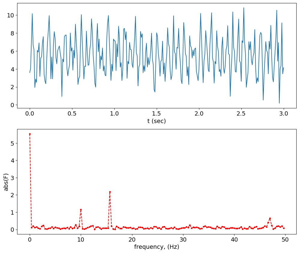
fig,ax = plt.subplots(2,1)
ax[0].plot(t,g)
ax[0].set_xlabel('t (sec)')
ax[1].set_ylabel('E (volts)')

ax[1].plot(Freq,A,'r--.')
# plot(frequency_2,Magnitude_Hann_2[:frequency_2.shape[0]], 'r-s')
ax[1].set_xlabel('frequency, (Hz)')
ax[1].set_ylabel('abs(F)')

Text(0, 0.5, 'abs(F)')

# windowing

N_2 = int(2**np.fix(np.log2(N)))  #total useful number of data points
T_2 = N_2/f_s  #total useful sample time (s)
del_f_2 = 1/T_2  #(Hz)
N_freq_2 = N_2/2  #number of useful discrete frequencies

t_2 = np.arange(0.0,T_2,del_t)  #time, t (s)
frequency_2 = np.arange(0,f_fold,del_f_2)  #frequency (Hz)
len2, = t_2.shape


g = g[:len2] # crop only the relevant sampled signal (original is longer)

DC_2 = np.mean(g)  #DC = mean value of input signal (V) (average of all the useful data)
g_uncoupled_2 = g - DC_2  #uncoupled

# Hanning window
u_Hann_2 = 0.5*(1-np.cos(2*np.pi*t_2/T_2))

# multiply in the time domain or convolute in frequency domain
g_Hann_2 = g_uncoupled_2*u_Hann_2 

# FFT of the windowed time signal 
G_Hann_2 = fft.fft(g_Hann_2,N_2) 

# get out the amplitude, return DC
# Correct for the Hanning window amplitude |F|*sqrt(8/3)/(N/2)
Magnitude_Hann_2 = np.abs(G_Hann_2)*np.sqrt(8./3.)/(N_2/2) 

#(also divide the first one by 2, and add back the DC value)
Magnitude_Hann_2[0] = Magnitude_Hann_2[0]/2 + DC_2  

len_loc, = Magnitude_Hann_2.shape
A_2 = Magnitude_Hann_2[0:int(round(len_loc/2))]
Freq_2 = frequency_2[0:int(round(len_loc/2))]

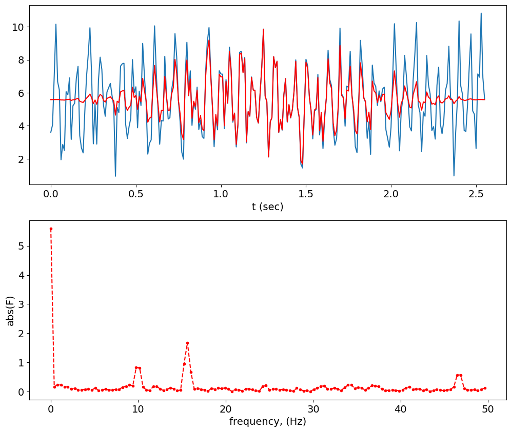
fig,ax = plt.subplots(2,1)
ax[0].plot(t_2,g)
ax[0].plot(t_2,g_Hann_2+DC_2,'r')
ax[0].set_xlabel('t (sec)')
ax[1].set_ylabel('E (volts)')

ax[1].plot(Freq_2,A_2,'r--.')
# plot(frequency_2,Magnitude_Hann_2[:frequency_2.shape[0]], 'r-s')
ax[1].set_xlabel('frequency, (Hz)')
ax[1].set_ylabel('abs(F)');

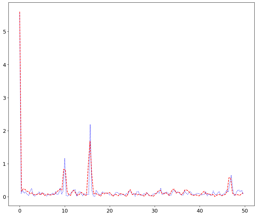
plt.plot(Freq,A,'b:',Freq_2,A_2,'r--')

[<matplotlib.lines.Line2D at 0x7fdeb1af1fd0>,
 <matplotlib.lines.Line2D at 0x7fdeb1afe100>]