This notebook presents the content of the SWGDRUG document as three distinct uncertainty budget examples.

Measurement Uncertainty Budget Examples (SWGDRUG SD-3)¶

This notebook details three examples of uncertainty budget calculations following the principles of the Guide to the Expression of Uncertainty in Measurement (GUM), as outlined in the SWGDRUG Supplemental Document SD-3.

General GUM Formulas¶

Standard Uncertainty ( $\boldsymbol{u_i}$ )¶

Individual uncertainty components ( $\pm a_i$ ) are converted to a standard uncertainty ( $u_i$ ) by dividing by a factor based on its probability distribution.

u_i = \frac{a_i}{\text{Divisor}}

(1)

Distribution Type	Divisor	Use Case
Rectangular (Uniform)	$\sqrt{3} \approx 1.732$	Instrument resolution, tolerances, etc.
Normal (Gaussian)	$k$ (Coverage Factor)	Calibration certificates where $U$ is given, or Type A standard deviation.

Combined Standard Uncertainty ( $\boldsymbol{u_c}$ )¶

For independent components, the combined standard uncertainty is the Root Sum of Squares (RSS) of the individual standard uncertainties.

u_c = \sqrt{u_1^2 + u_2^2 + \dots + u_n^2} = \sqrt{\sum_{i=1}^{N} u_i^2}

(2)

Expanded Uncertainty ( $\boldsymbol{U}$ )¶

The final reported uncertainty is the expanded uncertainty, calculated using a coverage factor ( $k$ ), typically $k=2$ for approximately 95% confidence.

U = k \cdot u_c

(3)

Example 1: Mass Measurement Uncertainty Budget¶

This example calculates the uncertainty associated with weighing a mass ( $m$ ) on an analytical balance, with a target reading of $0.10000 \text{ g}$ .

A. Define Parameters¶

Source of Uncertainty	Limit ( $\boldsymbol{a_i}$ ) [g]	Divisor	Distribution
Resolution/Readability	$\pm 0.00005$	$\sqrt{3}$	Rectangular
Calibration Certificate	$\pm 0.00005$	$k=2$	Normal
Linearity	$\pm 0.00010$	$\sqrt{3}$	Rectangular
Drift	$\pm 0.00005$	$\sqrt{3}$	Rectangular

B. Python Calculation¶

import numpy as np
import pandas as pd
import matplotlib.pyplot as plt

# 1. Define limits (a_i) and divisors
a_readability = 0.00005
a_calibration = 0.00005
a_linearity = 0.00010
a_drift = 0.00005

div_readability = np.sqrt(3)
div_calibration = 2.0  # k=2 assumed for normal distribution on certificate
div_linearity = np.sqrt(3)
div_drift = np.sqrt(3)

# 2. Calculate Standard Uncertainty (u_i)
u_readability = a_readability / div_readability
u_calibration = a_calibration / div_calibration
u_linearity = a_linearity / div_linearity
u_drift = a_drift / div_drift

# 3. Calculate Combined Standard Uncertainty (u_c)
u_c_mass = np.sqrt(u_readability**2 + u_calibration**2 + u_linearity**2 + u_drift**2)

# 4. Calculate Expanded Uncertainty (U)
k = 2.0
U_mass = k * u_c_mass

print(f"--- Mass Uncertainty Budget (g) ---")
print(f"Standard Uncertainty from Readability: {u_readability:.7f} g")
print(f"Standard Uncertainty from Calibration: {u_calibration:.7f} g")
print(f"Standard Uncertainty from Linearity:   {u_linearity:.7f} g")
print(f"Standard Uncertainty from Drift:       {u_drift:.7f} g")
print("-" * 40)
print(f"Combined Standard Uncertainty (u_c): {u_c_mass:.7f} g")
print(f"Expanded Uncertainty (U, k={k}):    {U_mass:.7f} g")

--- Mass Uncertainty Budget (g) ---
Standard Uncertainty from Readability: 0.0000289 g
Standard Uncertainty from Calibration: 0.0000250 g
Standard Uncertainty from Linearity:   0.0000577 g
Standard Uncertainty from Drift:       0.0000289 g
----------------------------------------
Combined Standard Uncertainty (u_c): 0.0000750 g
Expanded Uncertainty (U, k=2.0):    0.0001500 g

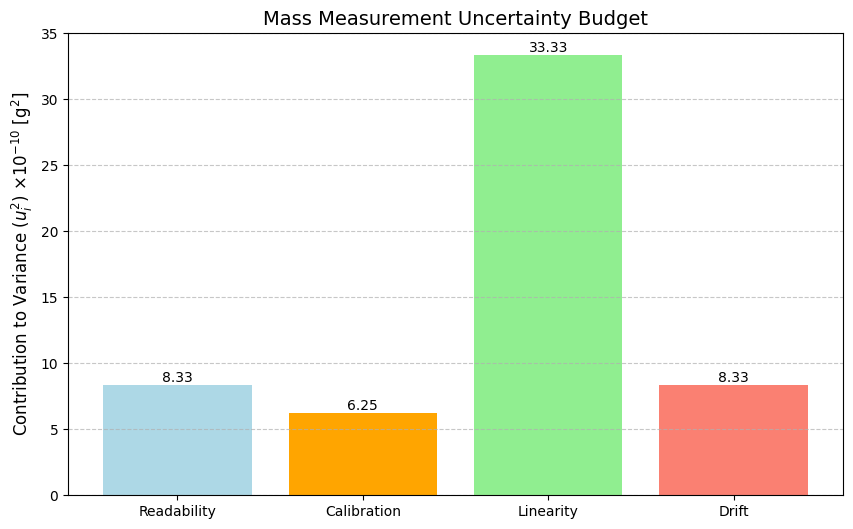
C. Uncertainty Budget Graph¶

# Create a DataFrame for plotting the budget
mass_data = {
    'Source': ['Readability', 'Calibration', 'Linearity', 'Drift'],
    'u_i': [u_readability, u_calibration, u_linearity, u_drift]
}
df_mass = pd.DataFrame(mass_data)
df_mass['Contribution (u_i^2)'] = df_mass['u_i']**2

# Plotting the contribution (variance)
plt.figure(figsize=(10, 6))
bars = plt.bar(df_mass['Source'], df_mass['Contribution (u_i^2)'] * 1e10, color=['lightblue', 'orange', 'lightgreen', 'salmon'])

plt.ylabel(r'Contribution to Variance ($u_i^2$) $\times 10^{-10}$ [$\mathrm{g}^2$]', fontsize=12)
plt.title('Mass Measurement Uncertainty Budget', fontsize=14)
plt.grid(axis='y', linestyle='--', alpha=0.7)

# Add text labels on bars
for bar in bars:
    yval = bar.get_height()
    plt.text(bar.get_x() + bar.get_width()/2, yval + 0.01, f'{yval:.2f}', ha='center', va='bottom', fontsize=10)

plt.show()

Example 2: Volume Measurement Uncertainty Budget¶

This example calculates the uncertainty associated with the volume ( $V$ ) delivered by a $5 \text{ mL}$ volumetric flask at a target temperature of $20 \text{ °C}$ .

A. Define Parameters¶

Source of Uncertainty	Limit ( $\boldsymbol{a_i}$ ) [mL]	Divisor	Distribution	Notes
Calibration Certificate	$\pm 0.003$	$k=2$	Normal	From certificate’s $U$ .
Temperature	$\pm 0.00085$	$\sqrt{3}$	Rectangular	Calculated uncertainty due to thermal expansion and $\Delta T$ .

B. Python Calculation¶

# 1. Define limits (a_i) and divisors
a_cal_vol = 0.003
a_temp_vol = 0.00085  # This value is based on the final uncertainty of the volume measurement

div_cal_vol = 2.0
div_temp_vol = np.sqrt(3)

# 2. Calculate Standard Uncertainty (u_i)
u_cal_vol = a_cal_vol / div_cal_vol
u_temp_vol = a_temp_vol / div_temp_vol

# 3. Calculate Combined Standard Uncertainty (u_c)
u_c_volume = np.sqrt(u_cal_vol**2 + u_temp_vol**2)

# 4. Calculate Expanded Uncertainty (U)
k = 2.0
U_volume = k * u_c_volume

print(f"--- Volume Uncertainty Budget (mL) ---")
print(f"Standard Uncertainty from Calibration: {u_cal_vol:.7f} mL")
print(f"Standard Uncertainty from Temperature: {u_temp_vol:.7f} mL")
print("-" * 40)
print(f"Combined Standard Uncertainty (u_c): {u_c_volume:.7f} mL")
print(f"Expanded Uncertainty (U, k={k}):    {U_volume:.7f} mL")

--- Volume Uncertainty Budget (mL) ---
Standard Uncertainty from Calibration: 0.0015000 mL
Standard Uncertainty from Temperature: 0.0004907 mL
----------------------------------------
Combined Standard Uncertainty (u_c): 0.0015782 mL
Expanded Uncertainty (U, k=2.0):    0.0031565 mL

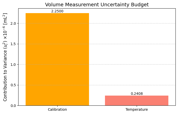
C. Uncertainty Budget Graph¶


# Create a DataFrame for plotting the budget
volume_data = {
    'Source': ['Calibration', 'Temperature'],
    'u_i': [u_cal_vol, u_temp_vol]
}
df_volume = pd.DataFrame(volume_data)
df_volume['Contribution (u_i^2)'] = df_volume['u_i']**2

# Plotting the contribution (variance)
plt.figure(figsize=(8, 5))
bars = plt.bar(df_volume['Source'], df_volume['Contribution (u_i^2)'] * 1e6, color=['orange', 'salmon'])

plt.ylabel(r'Contribution to Variance ($u_i^2$) $\times 10^{-6}$ [$\mathrm{mL}^2$]', fontsize=12)
plt.title('Volume Measurement Uncertainty Budget', fontsize=14)
plt.grid(axis='y', linestyle='--', alpha=0.7)

# Add text labels on bars
for bar in bars:
    yval = bar.get_height()
    plt.text(bar.get_x() + bar.get_width()/2, yval + 0.0001, f'{yval:.4f}', ha='center', va='bottom', fontsize=10)

plt.show()

Example 3: Concentration of a Standard Solution¶

This example calculates the uncertainty of the concentration ( $C$ ) of a solution prepared by dissolving the mass ( $m$ ) from Example 1 into the volume ( $V$ ) from Example 2.

The mathematical model for concentration is a quotient:

C = \frac{m}{V}

(4)

For models involving multiplication and division, it is standard practice to calculate the relative combined standard uncertainty ( $\frac{u_c(C)}{C}$ ) and then convert back to absolute uncertainty.

A. Relative Uncertainty Formulas ( $\LaTeX$ )¶

The relative combined standard uncertainty is given by the formula:

\frac{u_c(C)}{C} = \sqrt{\left(\frac{u(m)}{m}\right)^2 + \left(\frac{u(V)}{V}\right)^2}

(5)

The absolute combined standard uncertainty is then:

u_c(C) = C \cdot \frac{u_c(C)}{C}

(6)

B. Define Parameters (from Examples 1 and 2)¶

Mass ( $m$ ): $0.10000 \text{ g}$
Standard Uncertainty of Mass ( $\boldsymbol{u(m)}$ ): $u_{c\_mass} = 0.000085 \text{ g}$ (from Ex 1)
Volume ( $V$ ): $5.000 \text{ mL}$
Standard Uncertainty of Volume ( $\boldsymbol{u(V)}$ ): $u_{c\_volume} = 0.001584 \text{ mL}$ (from Ex 2)

C. Python Calculation¶

# 1. Define input values and their standard uncertainties
m = 0.10000      # Mass (g)
V = 5.000        # Volume (mL)
u_m = u_c_mass   # Combined standard uncertainty of mass (g)
u_V = u_c_volume # Combined standard uncertainty of volume (mL)

# 2. Calculate the Concentration (C)
C = m / V

# 3. Calculate Relative Standard Uncertainties
rel_u_m = u_m / m
rel_u_V = u_V / V

# 4. Calculate Relative Combined Standard Uncertainty (rel_u_c_C)
rel_u_c_C = np.sqrt(rel_u_m**2 + rel_u_V**2)

# 5. Calculate Absolute Combined Standard Uncertainty (u_c_C)
u_c_C = C * rel_u_c_C

# 6. Calculate Expanded Uncertainty (U_C)
k = 2.0
U_C = k * u_c_C

print(f"--- Concentration Uncertainty Budget (g/mL) ---")
print(f"Concentration (C): {C:.5f} g/mL")
print("-" * 40)
print(f"Relative u(m): {rel_u_m:.5f} (0.0{rel_u_m*100:.3f} %)")
print(f"Relative u(V): {rel_u_V:.5f} (0.0{rel_u_V*100:.3f} %)")
print("-" * 40)
print(f"Relative Combined Standard Uncertainty: {rel_u_c_C:.5f}")
print(f"Absolute Combined Standard Uncertainty (u_c): {u_c_C:.7f} g/mL")
print(f"Expanded Uncertainty (U, k={k}):    {U_C:.7f} g/mL")

--- Concentration Uncertainty Budget (g/mL) ---
Concentration (C): 0.02000 g/mL
----------------------------------------
Relative u(m): 0.00075 (0.00.075 %)
Relative u(V): 0.00032 (0.00.032 %)
----------------------------------------
Relative Combined Standard Uncertainty: 0.00081
Absolute Combined Standard Uncertainty (u_c): 0.0000163 g/mL
Expanded Uncertainty (U, k=2.0):    0.0000325 g/mL

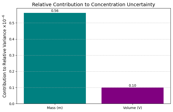
D. Relative Contribution Graph¶

This graph shows which input quantity (mass or volume) contributes the most to the overall uncertainty of the concentration.

# Create a DataFrame for plotting the relative contribution
concentration_data = {
    'Source': ['Mass (m)', 'Volume (V)'],
    'Relative u_i': [rel_u_m, rel_u_V]
}
df_conc = pd.DataFrame(concentration_data)
df_conc['Contribution to Relative Variance'] = df_conc['Relative u_i']**2

# Plotting the contribution (relative variance)
plt.figure(figsize=(8, 5))
bars = plt.bar(df_conc['Source'], df_conc['Contribution to Relative Variance'] * 1e6, color=['teal', 'purple'])

plt.ylabel(r'Contribution to Relative Variance $\times 10^{-6}$', fontsize=12)
plt.title('Relative Contribution to Concentration Uncertainty', fontsize=14)
plt.grid(axis='y', linestyle='--', alpha=0.7)

# Add text labels on bars
for bar in bars:
    yval = bar.get_height()
    plt.text(bar.get_x() + bar.get_width()/2, yval + 0.001, f'{yval:.2f}', ha='center', va='bottom', fontsize=10)

plt.show()

Measurement Uncertainty Budget Examples (SWGDRUG SD-3)

Measurement Uncertainty Budget Examples (SWGDRUG SD-3)¶

General GUM Formulas¶

Standard Uncertainty (ui\boldsymbol{u_i}ui​)¶

Combined Standard Uncertainty (uc\boldsymbol{u_c}uc​)¶

Expanded Uncertainty (U\boldsymbol{U}U)¶

Example 1: Mass Measurement Uncertainty Budget¶

A. Define Parameters¶

B. Python Calculation¶

C. Uncertainty Budget Graph¶

Example 2: Volume Measurement Uncertainty Budget¶

A. Define Parameters¶

B. Python Calculation¶

C. Uncertainty Budget Graph¶

Example 3: Concentration of a Standard Solution¶

A. Relative Uncertainty Formulas (LaTeX\LaTeXLATE​X)¶

B. Define Parameters (from Examples 1 and 2)¶

C. Python Calculation¶

D. Relative Contribution Graph¶

Standard Uncertainty ( $\boldsymbol{u_i}$ )¶

Combined Standard Uncertainty ( $\boldsymbol{u_c}$ )¶

Expanded Uncertainty ( $\boldsymbol{U}$ )¶

A. Relative Uncertainty Formulas ( $\LaTeX$ )¶