Static Calibration Errors: Engineering Testing & Measurements
This notebook demonstrates the application of the Guide to the Expression of Uncertainty in Measurement (GUM) framework for static calibration errors in two examples: an Orifice Flow Meter and a Cylindrical Storage Tank.
 |  |
Part 1: Calibration Example: Orifice Flow Meter
1.1 Orifice Flow Meter Theory
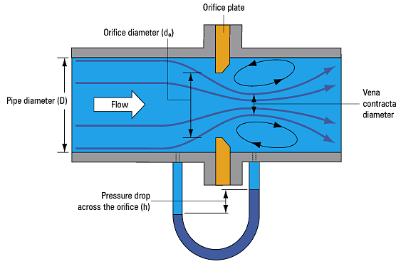
The flow rate through an orifice plate is determined by several measured quantities. The relationship is governed by the following formulae:
1. Ratio of the orifice diameter to the pipe diameter ():
2. Volumetric Flow Rate ():
The formula for the mass flow rate (in ) based on the pressure drop is given by:
Where:
: Discharge coefficient (accounts for friction)
: Expansibility factor (for compressible fluids)
: Pipe diameter
: Orifice diameter
: Fluid density
: Pressure drop across the orifice (in )
1.2 Input Values and Uncertainties
The following values and their corresponding Expanded Uncertainties () are provided for the flow meter calibration (Slides 4 and 5). Note that for calculations, we convert from to ( base unit).
| Quantity () | Symbol | Value () | Units | Expanded Uncertainty () | Coverage Factor () |
|---|---|---|---|---|---|
| Discharge coefficient | 0.6 | - | 0.003 | 2.0 | |
| Expansibility factor | 0.997 | - | 0.00027 | 2.0 | |
| Pipe diameter | 0.5 | 0.0001 | 1.73 | ||
| Orifice diameter | 0.3 | 0.00001 | 1.73 | ||
| Pressure drop | 50.0 | 100 | 2.0 | ||
| Density | 48.7 | 0.146 | 2.0 |
Python Setup and Variable Initialization
We will use the given values to calculate the flow rate and its associated combined standard uncertainty .
import numpy as np

# --- Input Values (Slide 4) ---
C = 0.6          # Discharge coefficient
epsilon = 0.997  # Expansibility factor
d1 = 0.5         # Pipe diameter (m)
d2 = 0.3         # Orifice diameter (m)
delta_p_kPa = 50.0
delta_p = delta_p_kPa * 1000 # Convert to Pa (50,000 Pa)
rho = 48.7       # Density (kg/m^3)
pi = np.pi

# --- Expanded Uncertainties U and Coverage Factors k (Slide 5 & 6) ---
U_C = 0.003; k_C = 2.0
U_epsilon = 0.00027; k_epsilon = 2.0
U_d1 = 0.0001; k_d1 = 1.73
U_d2 = 0.00001; k_d2 = 1.73
U_delta_p = 100; k_delta_p = 2.0 # U for delta_p in Pa
U_rho = 0.146; k_rho = 2.0
1.3 Flow Rate Calculation
First, calculate the diameter ratio and the theoretical flow rate .
# 1. Calculate diameter ratio beta
beta = d2 / d1
beta_squared = beta**2
beta_fourth = beta**4

# 2. Calculate Flow Rate Q (Calibrated Flow Rate from Slide 4 is 100.0 kg/s)
# Q = [C / sqrt(1 - beta^4)] * [epsilon * pi/4 * d1^2] * [sqrt(2 * rho * delta_p)]
Q_term1 = C / np.sqrt(1 - beta_fourth)
Q_term2 = epsilon * (pi/4) * d1**2
Q_term3 = np.sqrt(2 * rho * delta_p)

Q = Q_term1 * Q_term2 * Q_term3

print(f"Beta (β): {beta:.3f}")
print(f"Calculated Flow Rate (Q): {Q:.1f} kg/s")
# Note: The calculated value (100.0 kg/s) matches the Calibrated Flow Rate in Slide 4.
1.4 Uncertainty Budget (GUM Framework)
The combined standard uncertainty is calculated using the formula:
Where:
: Standard uncertainty for input quantity ().
: Sensitivity coefficient ()
: Uncertainty contribution to .
The table below (from Slide 6) summarizes the step-by-step calculation.
| Quantity | Value () | ||||||
|---|---|---|---|---|---|---|---|
| 0.6 | 0.003 | 2 | 0.0015 | 167 | 0.25 | 0.0628 | |
| 0.997 | 0.00027 | 2 | 0.00013 | 100 | 0.0135 | 0.0002 | |
| 0.5 | 0.0001 | 1.73 | -60 | -0.0035 | |||
| 0.3 | 0.00001 | 1.73 | 766 | 0.0044 | |||
| 100 | 2 | 50 | 0.001 | 0.05 | 0.0025 | ||
| 48.7 | 0.146 | 2 | 0.07305 | 1.03 | 0.075 | 0.0057 | |
| 100.0 | 0.533 | 2 | 0.267 | 1 | 0.267 | 0.0711 |
Calculations based on the Table
We can verify the combined uncertainty by summing the squared contributions.
# --- Standard Uncertainties (u = U/k) ---
u_C = U_C / k_C
u_epsilon = U_epsilon / k_epsilon
u_d1 = U_d1 / k_d1
u_d2 = U_d2 / k_d2
u_delta_p = U_delta_p / k_delta_p
u_rho = U_rho / k_rho

# --- Sensitivity Coefficients (c) from the table (Slide 6) ---
c_C = 167
c_epsilon = 100
c_d1 = -60
c_d2 = 766
c_delta_p = 0.001
c_rho = 1.03

# --- Squared Uncertainty Contributions (u*c)^2 from the table (Slide 6) ---
uc2_C = 0.0628
uc2_epsilon = 0.0002
uc2_d1 = 1.20E-5
uc2_d2 = 1.96E-5
uc2_delta_p = 0.0025
uc2_rho = 0.0057

# --- 7. Calculate Combined Squared Uncertainty Summation ---
sum_uc_squared = uc2_C + uc2_epsilon + uc2_d1 + uc2_d2 + uc2_delta_p + uc2_rho

# --- 8. Calculate Combined Standard Uncertainty (u_c) ---
u_c_Q = np.sqrt(sum_uc_squared)

# --- Final Expanded Uncertainty (U_Q) ---
# The table uses k=2 for the final Expanded Uncertainty (U = k * u_c).
k_final = 2
U_Q = k_final * u_c_Q

print(f"Sum of Squared Contributions (Σ(u·c)²): {sum_uc_squared:.4f} (Matches 0.0711 from table)")
print(f"Combined Standard Uncertainty (u_c): {u_c_Q:.3f} (Matches 0.267 from table)")
print(f"Expanded Uncertainty (U) for Q (k=2): {U_Q:.3f} (Matches 0.533 from table)")

# Final result for the flow rate: Q = 100.0 ± 0.533 kg/s (k=2)
Part 2: Calibration Example: Cylindrical Storage Tank
2.1 Volume and Thermal Expansion
The second example deals with calculating the volume of a cylindrical storage tank.
1. Governing Equation for Volume ():
Where:
: Diameter
: Height
2. Thermal Expansion Correction:
If the measurement is taken at a temperature different from a standard reference temperature (e.g., ), a correction for thermal expansion must be applied to the measured volume .
Where is the cubical expansion coefficient. This correction introduces two new uncertainty sources: and .
2.2 Uncertainty Budget (Uncorrelated Measurements)
This section examines the uncertainty budget for the final corrected volume, assuming all measurement sources are uncorrelated.
| Source | ||||||
|---|---|---|---|---|---|---|
| Calibration (Diameter) | 0.048 | 2.00 | 0.024 | 39.96 | 0.955 | 0.920 |
| Determination (Diameter) | - | - | 0.021 | 39.96 | 0.839 | 0.704 |
| Time drift (Diameter) | 0.005 | 1.73 | 0.003 | 39.96 | 0.115 | 0.013 |
| Calibration (Height) | 0.100 | 2.00 | 0.050 | 18.10 | 0.905 | 0.819 |
| Resolution (Height) | 0.026 | 1.73 | 0.015 | 18.10 | 0.272 | 0.074 |
| Time drift (Height) | 0.010 | 1.73 | 0.006 | 18.10 | 0.104 | 0.011 |
| Temperature () | 0.550 | 2.00 | 0.275 | -0.004 | -0.001 | |
| Cubical Expansion () | 1.73 | -1437 | -0.002 | |||
| Volume () | 3.188 | 2.00 | 1.594 | 1 | 1.594 | 2.541 |
In the uncorrelated case, the combined standard uncertainty is calculated by taking the square root of the sum of the values in the column (Total sum 2.541).
The Expanded Uncertainty is then calculated with :
2.3 Uncertainty Budget (Correlated Measurements)
When measurements are correlated, the uncertainty propagation formula must include a covariance term. For the correlation between two input quantities and with correlation coefficient :
The presentation (Slide 10) shows the result when some measurements are considered correlated. A key example is often the correlation between the Calibration of Diameter and the Calibration of Height, as both might rely on the same potentially flawed reference standard.
| Source | ||||||
|---|---|---|---|---|---|---|
| Calibration (Diameter) | 0.048 | 2.00 | 0.024 | 39.96 | - | |
| ... | ... | ... | ... | ... | ... | ... |
| Calibration (Height) | 0.100 | 2.00 | 0.050 | 18.10 | ||
| ... | ... | ... | ... | ... | ... | ... |
| Volume () | 4.136 | 2.00 | 2.068 | 1 | 2.068 | 4.277 |
Key Observation:
The squared uncertainty for the Calibration (Height) is now 3.475, which is much larger than its uncorrelated value (0.819). This large value in the column often represents the combined sum of the individual squared contribution plus the covariance term .
The final result for the Volume’s expanded uncertainty increased from 3.188 to 4.136.
Conclusion on Correlation: Including correlation, even for a few key sources, can significantly increase the total combined uncertainty of the final result.
Part 3: Typical Calibration Report
A typical calibration report (like the example for the ICP Accelerometer) provides essential information for uncertainty analysis, including:
Calibration Data: Key measured characteristics (e.g., Voltage Sensitivity, Transverse Sensitivity, Output Bias Level).
Key Specifications: Operational parameters (e.g., Range, Resolution, Time Constant).
Frequency Response: A plot or table showing the deviation of the measured characteristic (e.g., Amplitude Deviation) across a range of frequencies. This information is crucial for dynamic, non-static error analysis.