Calibration of non-linear relations#
Non linear relations of \(y = f(x)\)#
When we expect $\(y = ax^2 + bx + c\)\(, our task is to estimate \)a, b, c$ using the best-fit, i.e that coefficients that give us the smallest error between the the model and the measurements.
In any case, the easiest and most accurate fit is of a linear type - we know that the static sensitivity is our goal and it has a lot of usefuleness in the following measurements. Therefore we always look for the way to convert our non-linear relation to linear one and then perform best-fit or regression on the transformed variables.
%pylab inline
pylab.rcParams['figure.figsize'] = 10, 8
pylab.rcParams['font.size'] = 16

# read the data
import numpy as np
x = np.array([0.5, 1.0, 2.0, 5.0, 10.0, 20.0, 50.0, 100.0]) # cm
y = np.array([0.4, 1.0, 2.3, 6.9, 15.8, 36.4, 110.1, 253.2]) # Volt
%pylab is deprecated, use %matplotlib inline and import the required libraries.
Populating the interactive namespace from numpy and matplotlib
fig = figure()
plot(x,y,'o:')
xlim(-5,110)
ylim(-5,300)
xlabel('$x$ [cm]')
ylabel('$y$ [V]')
Text(0, 0.5, '$y$ [V]')
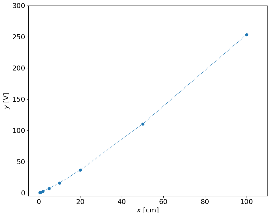
Conclusion:#
Obviously the result is non-linear and the best sensitivity we can get is between 20 and 40 cm, but not for small distances
If the relationship is a known function and it’s a physically relevant one, we could use it to show that distance to voltage should be related as a power law and not really linearly. Let’s check the logarithmic scale, since we know that:
\(\log y = \log (bx^m) = \log b + m \log x \)
fig = figure()
loglog(x,y,'o:')
# xlim(-5,110)
# ylim(-5,300)
xlabel('$x$ [cm]')
ylabel('$y$ [V]')
Text(0, 0.5, '$y$ [V]')
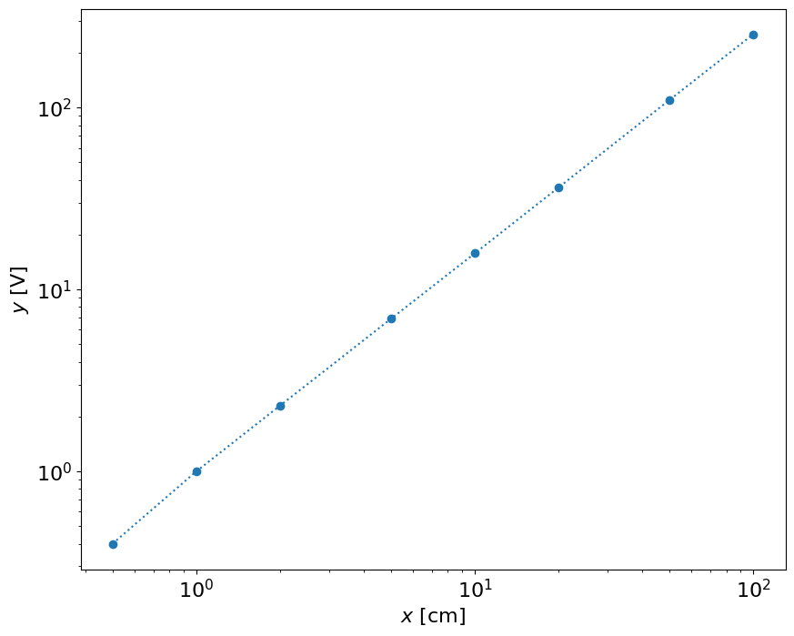
This result shows that the result is close to linear in the log-log space. Let’s do calibration in \(\log(x)\) and \(\log(y)\). It can be either \(\log\) or \(\log_{10}\)
fig = figure()
plot(log(x),log(y),'o:')
# xlim(-5,110)
# ylim(-5,300)
xlabel('$\log (x)$ [cm]')
ylabel('$\log (y) $ [V]')
<>:5: SyntaxWarning: invalid escape sequence '\l'
<>:6: SyntaxWarning: invalid escape sequence '\l'
<>:5: SyntaxWarning: invalid escape sequence '\l'
<>:6: SyntaxWarning: invalid escape sequence '\l'
/tmp/ipykernel_274764/86560295.py:5: SyntaxWarning: invalid escape sequence '\l'
  xlabel('$\log (x)$ [cm]')
/tmp/ipykernel_274764/86560295.py:6: SyntaxWarning: invalid escape sequence '\l'
  ylabel('$\log (y) $ [V]')
Text(0, 0.5, '$\\log (y) $ [V]')
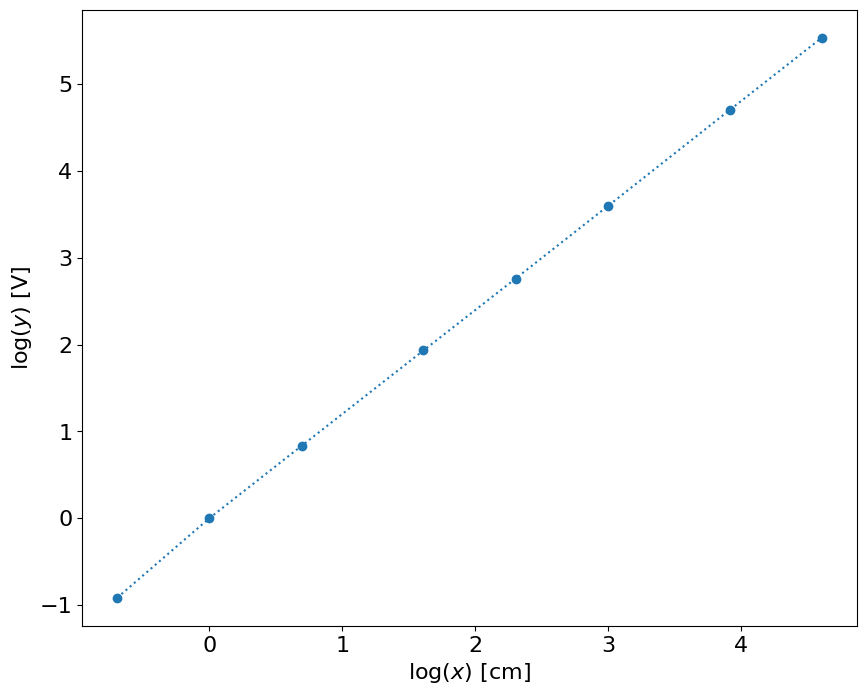
# linear fit
p = polyfit(log10(x),log10(y),1)
p
array([ 1.21031575, -0.01252781])
# let's check the fit:
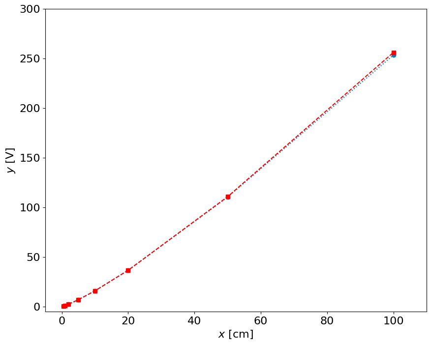
fig = figure()
yfit = 10**(p[0]*log10(x) + p[1])
plot(x,y,'o:',x,yfit,'rs--')
xlim(-5,110)
ylim(-5,300)
xlabel('$x$ [cm]')
ylabel('$y$ [V]')
Text(0, 0.5, '$y$ [V]')
how do we measure?#
measure the \(y\) [V], take a \(\log_{10}(y)\), estimate the \(\log_{10}(x) \) using the calibration curve:
\( \log_{10}(x) = (\log_{10}(y) + 0.0125)/1.21 \)
Note that we can use this function in the full input scale and full output scale, take:
\(10^{\log_{10} (x)}\)
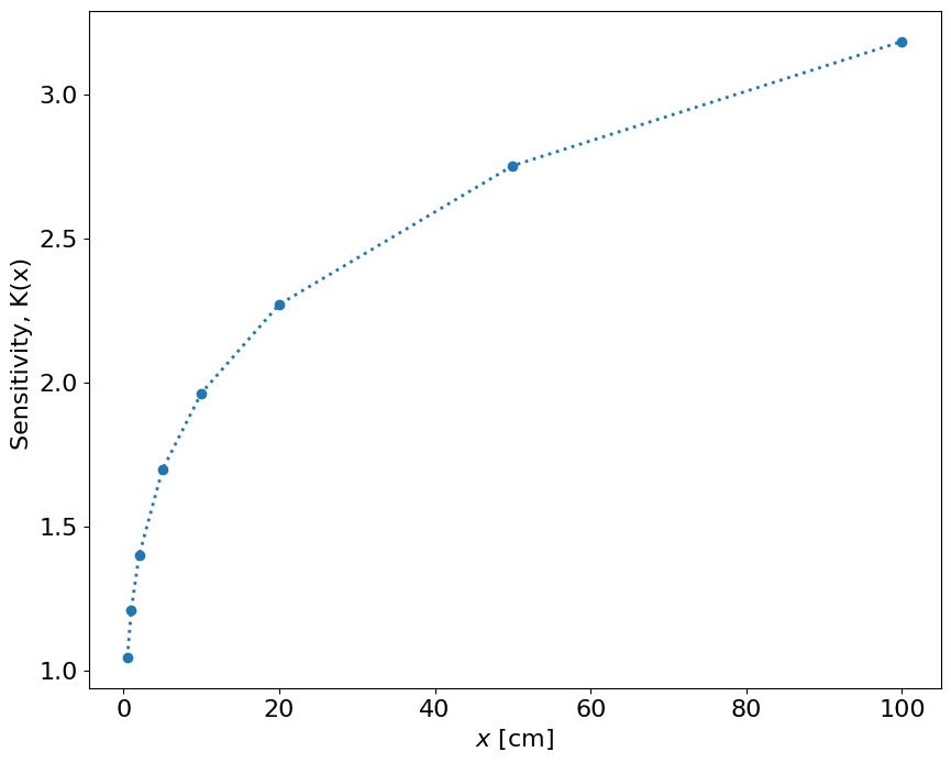
The sensitivity of this function is:
\(K(x) = dy/dx = d/dx ( x^{1.2} ) = 1.2 x^{0.2} \)
fig = figure()
K = 1.21*x**0.21
plot(x,K,'o:',lw=2)
xlabel('$x$ [cm]')
ylabel('Sensitivity, K(x) ')
Text(0, 0.5, 'Sensitivity, K(x) ')