This tutorial demonstrates the basics of Particle Image Velocimetry (PIV) analysis using OpenPIV. You’ll learn how to: - Load image pairs - Apply the PIV correlation algorithm - Validate and filter results - Visualize velocity fields
Theory
PIV is a non-intrusive flow measurement technique that calculates velocity fields from pairs of images captured at short time intervals. Particles seeded in the flow are tracked between two laser pulses, and their displacement provides velocity information.
Code Example
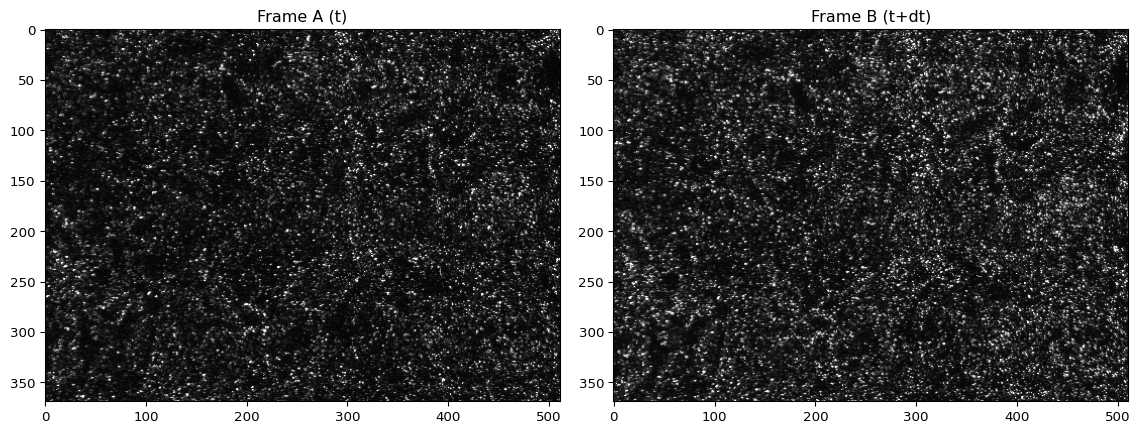
Let’s start by loading the test images and visualizing them:
import pathlibfrom openpiv import tools, pyprocess, validation, filters, scalingimport numpy as npimport matplotlib.pyplot as plt# Load the test images - use absolute path to the data folderrepo_root ="/home/user/Documents/GitHub/openpiv-python-examples/openpiv-tutorials/data/test1"frame_a = tools.imread(f"{repo_root}/exp1_001_a.bmp")frame_b = tools.imread(f"{repo_root}/exp1_001_b.bmp")# Display both framesfig, axes = plt.subplots(1, 2, figsize=(12, 8))axes[0].imshow(frame_a, cmap=plt.cm.gray)axes[0].set_title("Frame A (t)")axes[1].imshow(frame_b, cmap=plt.cm.gray)axes[1].set_title("Frame B (t+dt)")plt.tight_layout()plt.show()
Now let’s apply the PIV algorithm to find the displacement:
# Define PIV parameterswinsize =32# interrogation window size in pixelssearchsize =38# search area size in pixels overlap =12# overlap between windows (50%)dt =0.02# time between pulses (seconds)# Run the PIV analysisu0, v0, sig2noise = pyprocess.extended_search_area_piv( frame_a.astype(np.int32), frame_b.astype(np.int32), window_size=winsize, overlap=overlap, dt=dt, search_area_size=searchsize, sig2noise_method="peak2peak",)# Get the coordinate gridx, y = pyprocess.get_coordinates( image_size=frame_a.shape, search_area_size=searchsize, overlap=overlap)print(f"Velocity field shape: {u0.shape}")print(f"Number of vectors: {u0.size}")print(f"Signal-to-noise ratio range: {sig2noise.min():.2f} - {sig2noise.max():.2f}")
Velocity field shape: (13, 19)
Number of vectors: 247
Signal-to-noise ratio range: 0.00 - 2.66
Validate the results using signal-to-noise ratio:
# Validate using signal-to-noise ratioflags = validation.sig2noise_val(sig2noise, threshold=1.05)# Replace outliersu2, v2 = filters.replace_outliers( u0, v0, flags, method="localmean", max_iter=3, kernel_size=3)# Convert to physical unitsx_1, y_1, u3, v3 = scaling.uniform(x, y, u2, v2, scaling_factor=96.52)x_1, y_1, u3, v3 = tools.transform_coordinates(x_1, y_1, u3, v3)print(f"Validated vectors: {flags.sum()} / {flags.size}")print(f"Velocity range U: {u3.min():.2f} to {u3.max():.2f} pix/s")print(f"Velocity range V: {v3.min():.2f} to {v3.max():.2f} pix/s")
Validated vectors: 17 / 247
Velocity range U: -0.80 to 0.92 pix/s
Velocity range V: -3.54 to -2.12 pix/s
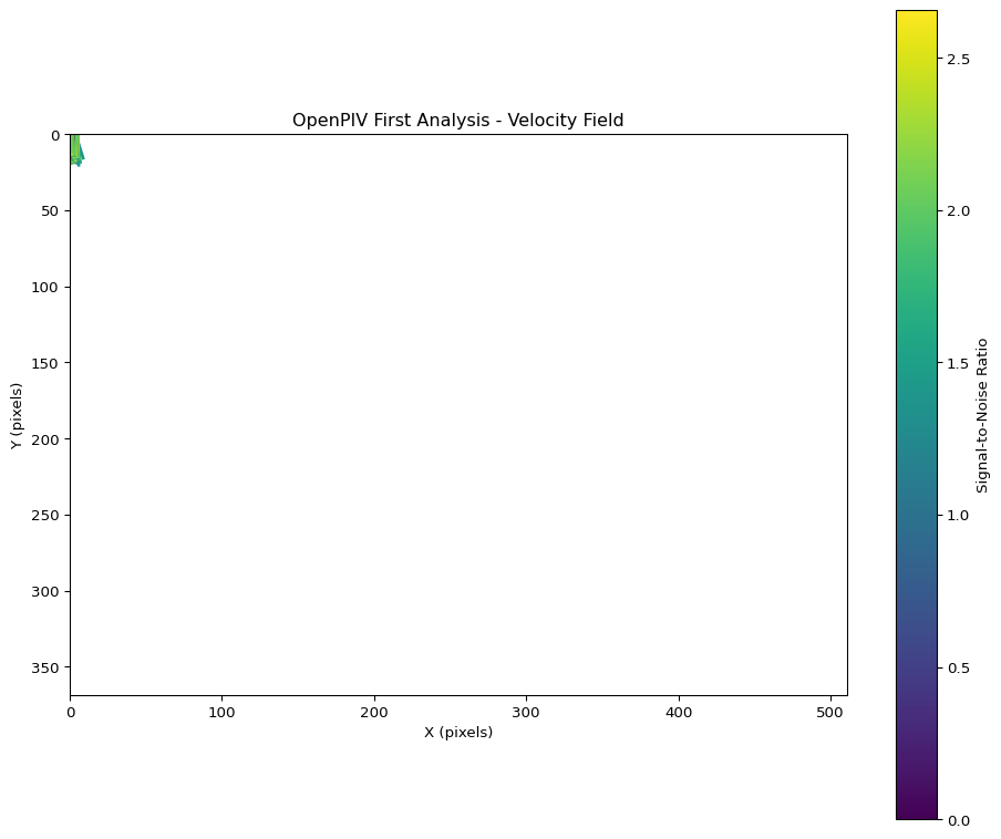
Visualize the velocity field:
# Display the vector field using quiver plotfig, ax = plt.subplots(figsize=(10, 8))Q = ax.quiver(x_1, y_1, u3, -v3, sig2noise, scale=50, pivot='middle')ax.set_aspect('equal')ax.invert_yaxis()ax.set_xlabel('X (pixels)')ax.set_ylabel('Y (pixels)')ax.set_title("OpenPIV First Analysis - Velocity Field")ax.set_xlim(0, frame_a.shape[1])ax.set_ylim(frame_a.shape[0], 0)plt.colorbar(Q, label='Signal-to-Noise Ratio')plt.tight_layout()plt.show()
Summary
In this tutorial you: 1. Loaded image pairs using OpenPIV tools 2. Applied the extended search area PIV algorithm 3. Validated results with signal-to-noise ratio filtering 4. Replaced outlier vectors using local mean filtering 5. Visualized the velocity field