import matplotlib.pyplot as plt
import numpy as np
%matplotlib inline

from numpy import fft

import matplotlib as mpl
mpl.rc('font', size=14)
mpl.rc('figure',figsize=(12,10))
# Given:
f_s = 100.0 # sampling frequency (Hz)
T = 3.0 # total actual sample time (s)
g = np.loadtxt('../data/FFT_Example_data_with_window.txt')
# add noise
for i in range(10):
g += np.random.rand(g.shape[0])# Calculate
N = f_s*T #total actual number of data points
del_t = 1./f_s #(s)
del_f = 1./T #(Hz)
f_fold = f_s/2. #folding frequency = max frequency of FFT (Hz)
N_freq = N/2. #number of discrete frequencies
t = np.arange(0.0,T+del_t,del_t) #time, t (s)
g += 1.2*np.sin(2*np.pi*10*t)frequency = np.arange(0,f_fold,del_f) #frequency (Hz)
G = fft.fft(g) # FFT
Magnitude = np.abs(G)/(N/2.) #|F|/(N/2)
Magnitude[0] = Magnitude[0]/2
len_loc, = Magnitude.shape
A = Magnitude[0:np.int(round(len_loc/2))]
Freq = frequency[0:np.int(round(len_loc/2))]/tmp/ipykernel_208438/2700199249.py:6: DeprecationWarning: `np.int` is a deprecated alias for the builtin `int`. To silence this warning, use `int` by itself. Doing this will not modify any behavior and is safe. When replacing `np.int`, you may wish to use e.g. `np.int64` or `np.int32` to specify the precision. If you wish to review your current use, check the release note link for additional information.
Deprecated in NumPy 1.20; for more details and guidance: https://numpy.org/devdocs/release/1.20.0-notes.html#deprecations
A = Magnitude[0:np.int(round(len_loc/2))]
/tmp/ipykernel_208438/2700199249.py:7: DeprecationWarning: `np.int` is a deprecated alias for the builtin `int`. To silence this warning, use `int` by itself. Doing this will not modify any behavior and is safe. When replacing `np.int`, you may wish to use e.g. `np.int64` or `np.int32` to specify the precision. If you wish to review your current use, check the release note link for additional information.
Deprecated in NumPy 1.20; for more details and guidance: https://numpy.org/devdocs/release/1.20.0-notes.html#deprecations
Freq = frequency[0:np.int(round(len_loc/2))]
fig,ax = plt.subplots(2,1)
ax[0].plot(t,g)
ax[0].set_xlabel('t (sec)')
ax[1].set_ylabel('E (volts)')

ax[1].plot(Freq,A,'r--.')
# plot(frequency_2,Magnitude_Hann_2[:frequency_2.shape[0]], 'r-s')
ax[1].set_xlabel('frequency, (Hz)')
ax[1].set_ylabel('abs(F)')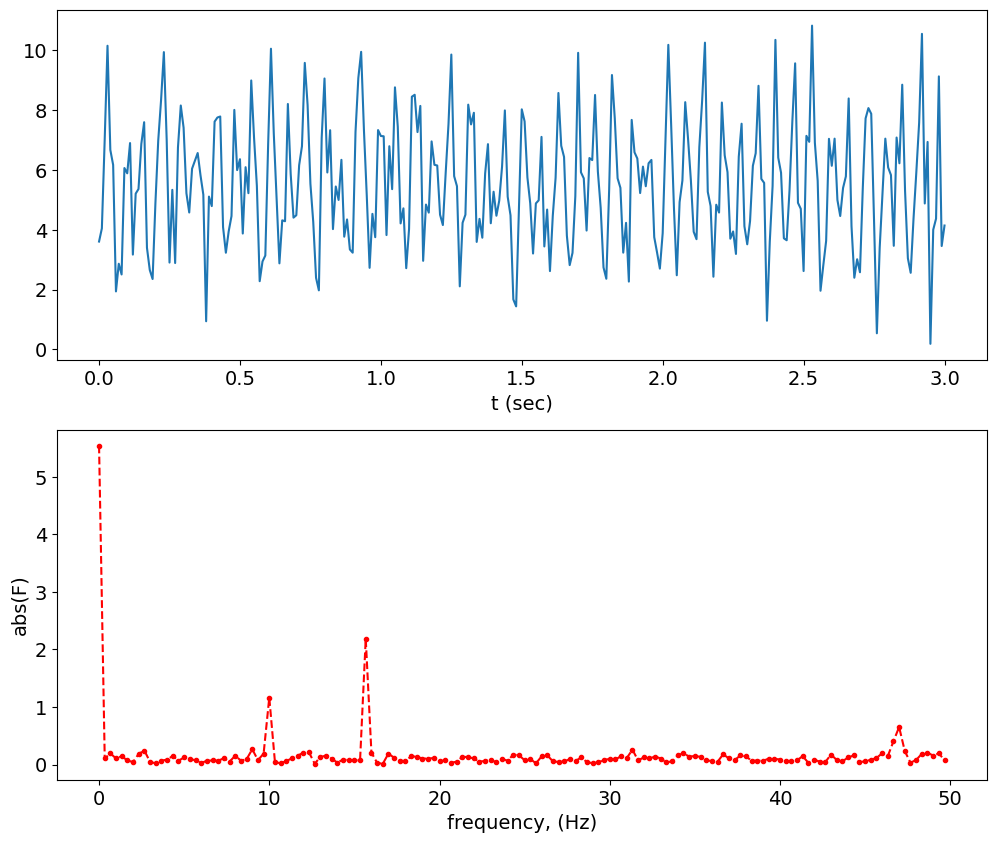
# windowing

N_2 = int(2**np.fix(np.log2(N)))  #total useful number of data points
T_2 = N_2/f_s  #total useful sample time (s)
del_f_2 = 1/T_2  #(Hz)
N_freq_2 = N_2/2  #number of useful discrete frequencies

t_2 = np.arange(0.0,T_2,del_t)  #time, t (s)
frequency_2 = np.arange(0,f_fold,del_f_2)  #frequency (Hz)
len2, = t_2.shape


g = g[:len2] # crop only the relevant sampled signal (original is longer)

DC_2 = np.mean(g)  #DC = mean value of input signal (V) (average of all the useful data)
g_uncoupled_2 = g - DC_2  #uncoupled

# Hanning window
u_Hann_2 = 0.5*(1-np.cos(2*np.pi*t_2/T_2))

# multiply in the time domain or convolute in frequency domain
g_Hann_2 = g_uncoupled_2*u_Hann_2

# FFT of the windowed time signal
G_Hann_2 = fft.fft(g_Hann_2,N_2)

# get out the amplitude, return DC
# Correct for the Hanning window amplitude |F|*sqrt(8/3)/(N/2)
Magnitude_Hann_2 = np.abs(G_Hann_2)*np.sqrt(8./3.)/(N_2/2)

#(also divide the first one by 2, and add back the DC value)
Magnitude_Hann_2[0] = Magnitude_Hann_2[0]/2 + DC_2

len_loc, = Magnitude_Hann_2.shape
A_2 = Magnitude_Hann_2[0:int(round(len_loc/2))]
Freq_2 = frequency_2[0:int(round(len_loc/2))]
fig,ax = plt.subplots(2,1)
ax[0].plot(t_2,g)
ax[0].plot(t_2,g_Hann_2+DC_2,'r')
ax[0].set_xlabel('t (sec)')
ax[1].set_ylabel('E (volts)')
ax[1].plot(Freq_2,A_2,'r--.')
# plot(frequency_2,Magnitude_Hann_2[:frequency_2.shape[0]], 'r-s')
ax[1].set_xlabel('frequency, (Hz)')
ax[1].set_ylabel('abs(F)');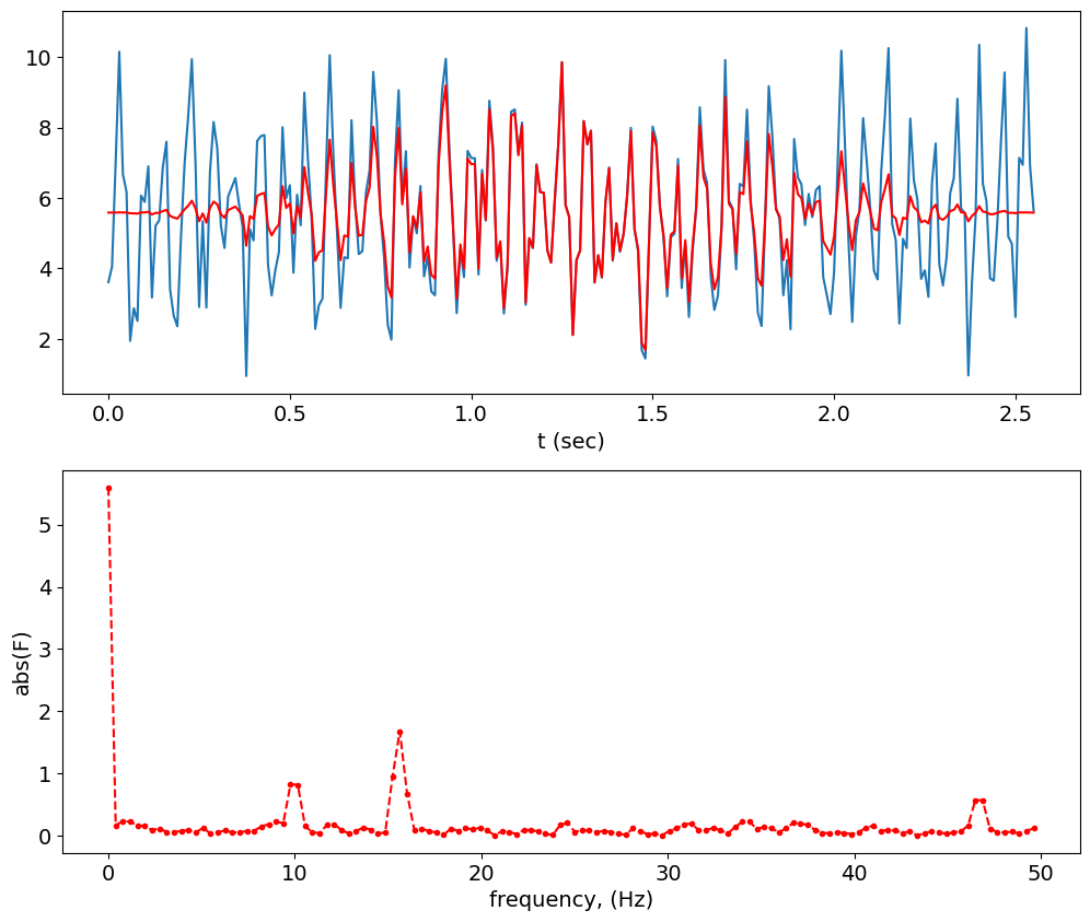
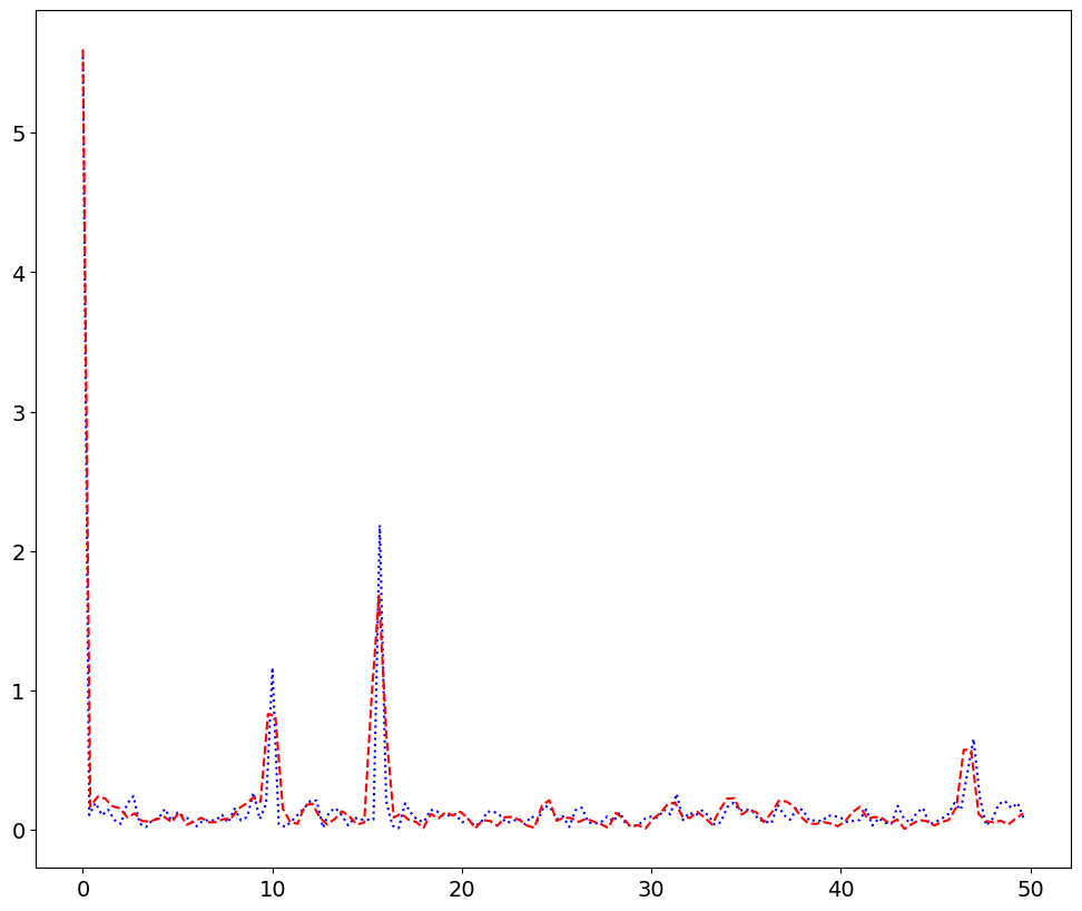
plt.plot(Freq,A,'b:',Freq_2,A_2,'r--')